

✨ TL;DR: We design a transformer-shaped module built around relaxation steps of a driven disordered spin system after an input “quench”. Taking one learned-initialization step $\approx$ a parallel transformer block, taking $\infty$ steps $\approx$ a deep-equilibrium module. A toy language-modeling training experiment shows that the one-step modules learn to use task-relevant transient states, and do not approach their fixed points.
Introduction
✨ GitHub repository:
mcbal/neqnn
Transformers are powerful driven dynamical systems, yet their internal computation is not often discussed in terms of nonequilibrium thermodynamics. Building on Spin-Model Transformers (2023), we construct a transformer-shaped module from the mean-field dynamics of a driven disordered vector-spin system, turning its forward pass into a controllable quench-and-relax process with explicit drive, relaxation, and learning timescales. This yields a design space spanning finite-step transformer-like, recurrent stateful, and fixed-point/deep-equilibrium-like computation, together with mean-field proxies for steady-state irreversibility and post-quench relaxation. We run numerical experiments to calibrate these approximations against stochastic simulations and show that, in a toy language model trained with a short relaxation horizon, useful computation is found in task-relevant transients rather than in underconverged fixed-point solutions.
Driving a spin-model transformer module
In this section, we design a minimal spin-model transformer module whose forward pass implements a controllable nonequilibrium quench-and-relax process. We identify three timescales and two dynamical regimes, leading to a natural categorization of the design space into stateless and stateful variations of transformer-like and deep-equilibrium-like architectures.
At the end of this section, we comment on the module’s relation to transformers. Below we already provide a cheat sheet mapping concepts between spin-model transformer modules and transformer modules. For a full overview of the symbols used in this post, see Appendix A.
| Spin-model analogue | Transformer component |
|---|---|
| Local drives $\mathbf{x}_{i,t}$ | Module inputs |
| “The drive” $\mathbf{X}_{t}$ | Current context window |
| Magnetizations $\mathbf{m}_{i,t}$ | Internal state and module outputs |
| Saturation of magnetization map $\varphi_{\beta}$ | Bounded response and normalization |
| Parameterized couplings $\mathbf{J}$ | Attention matrix |
| Learned initializer $\mathbf{M}_{t, 0} = \varphi_{\beta}\left(\mathbf{X}_{t}\mathbf{W}_{V}\right)$ | Initial state analogous to values in QKV attention |
| Head-specific coupling matrices $J^{(h)}(\mathbf{X}_{t})$ acting on separate subspaces or parallel vector-spin systems | Multihead attention |
A minimal controllable drive-conditioned system
In Spin-Model Transformers (2023) we showed how to apply dynamical mean-field theory to approximate the time-dependent behavior of asymmetric vector-spin models. We started from a spin system of $N$ vector spins $\mathbf{s}_{i,t} \in \mathbb{R}^{D}$ talking to each other via an $N \times N$ pairwise coupling matrix $J_{ij}$ with the underlying synchronous, parallel-updates stochastic dynamics characterized by a discrete-time Markov chain transition probability. External magnetic fields $\mathbf{x}_{i,t} \in \mathbb{R}^{D}$ bias the vector spins and act as local drives. We use the notation $\mathbf{A} \in \mathbb{R}^{N \times D}$ to refer to matrices of stacked vectors $\mathbf{a}_{i} \in \mathbb{R}^{D}$.
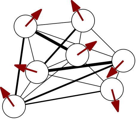
Our vector-spin system of interest is defined by a first-order Plefka[t-1,t]1 mean-field recurrence relation for its spin expectation values, or magnetizations
where $\beta$ denotes the inverse temperature and $R^2=D/2 -1$ is a length scale choice in the large-$D$ approximation2. The effective field
\begin{equation} \mathbf{h}_{i,t,k} = \mathbf{x}_{i,t} + f_{\boldsymbol{\theta}_{\mathrm{FFN}}}\left( \mathbf{x}_{i,t} \right) + \sum_{j} J_{ij} (\mathbf{X}_{t}) \mathbf{m}_{j,t,k} \end{equation}contains a parameterized drive-conditioned coupling rule3
\begin{equation} \mathbf{J} (\mathbf{X}_{t}) = \mathrm{softmax}\left( \alpha \mathbf{X}_{t} \boldsymbol{W}_{Q} \boldsymbol{W}_{K}^{T} \mathbf{X}_{t}^{T} \right), \label{eq:softmax} \end{equation}and a parameterized position-wise non-linear drive-conditioned field $f_{\boldsymbol{\theta}_{\mathrm{FFN}}}\left( \mathbf{x}_{i,t} \right)$ added to the local drive $\mathbf{x}_{i,t}$. The latter can be motivated as a learnable self-correction term in the style of the Thouless–Anderson–Palmer (TAP) approach. Each vector spin effectively experiences a local mean-field that is the sum of a residual stream drive, a feed-forward-like drive, and attention-like couplings. The time index $t$ tracks changes in the external drive while $k$ indexes an internal relaxation step.
By making the effective drive as well as the couplings depend on the drive $\mathbf{X}_{t}$, a sudden shift $\mathbf{X}_{t} \to \mathbf{X}_{t+1}$ changes both the local fields as well as the interactions and quenches the system into a new instantaneous dynamics4. During internal relaxation iterations, the drive $\mathbf{X}_{t}$ and the parameters $\boldsymbol{\theta} = \{ \mathbf{W}_{Q}, \mathbf{W}_{K}, \boldsymbol{\theta}_{\mathrm{FFN}} \}$ are held fixed.
Approximation stack: At the stochastic level, the process looks something like $P_{\boldsymbol{\theta}, \mathbf{X}_{t}}(\mathbf{S}_{t, k+1} | \mathbf{S}_{t, k}) = \prod^{N}_{i=1} \frac{\operatorname{exp}\left[\beta \mathbf{s}_{i,t,k+1} \cdot \mathbf{h}_{i,t,k} \right]}{Z\left(\mathbf{h}_{i,t,k}\right)}$ with effective field $\mathbf{h}_{i,t,k} = \mathbf{x}_{i,t} + f_{\boldsymbol{\theta}_{\mathrm{FFN}}}\left( \mathbf{x}_{i,t} \right) + \sum_{j} J_{ij} (\mathbf{X}_{t}) \mathbf{s}_{j,t,k}$ and single-site normalization constant $Z\left(\mathbf{h}\right)$. The product-form kernel assumes parallel, conditionally independent site updates. An asynchronous spin process would need a different kernel and should not be conflated with this one. The stochastic process is the thermodynamic object, and the magnetization recurrence used as the neural-network module is a Plefka mean-field approximation to its one-point dynamics. In the next sections, we will, among other quantities, discuss deterministic mean-field fixed-point magnetizations $\mathbf{M}^{\star}_{t}(\mathbf{X}_{t})$ which approximate one-point marginals of the stochastic steady state $\pi_{\mathbf{X_{t}}}$. It is useful to keep these levels of approximation in the back of your mind.
We end up with a highly reconfigurable system that is dynamically shaped by the drive. These drive dependencies enable the mean-field system to encode subtle correlational structures. The system’s parameters can be shaped through training in an outer optimization loop to make an already responsive system adaptive by controlling how the system responds, fluctuates, and relaxes after a quench.
Building modules: three clocks, slow plasticity, and two relaxation limits
Looking at Eq. \eqref{eq:paralleltransformer} we notice its close resemblance to the forward pass of a parallel transformer block. To make this more precise, we need to specify how to implement spin-model transformer modules in practice. What is up with this weird internal state and internal relaxation dimension? How can this system even serve as a neural network module?
Let us begin by writing the forward pass Eq. \eqref{eq:paralleltransformer} more generally as
\begin{equation} \mathbf{M}^{(\ell)}_{t, k+1} = F_{\boldsymbol{\theta}^{(\ell)}_{n}} \left( \mathbf{X}^{(\ell)}_{t}, \mathbf{M}^{(\ell)}_{t, k} \right) \end{equation}and clearly state the clocks involved:
- $k$ indexes fast internal relaxation within the module
- $t$ indexes changes in the environmental drive or input context
- $n$ indexes slow parameter updates $\boldsymbol{\theta}^{(\ell)}_{n+1} = \boldsymbol{\theta}^{(\ell)}_{n} - \eta \nabla_{\boldsymbol{\theta}^{(\ell)}} \mathcal{L}^{\ell}_{t}$ for some learning rate $\eta \ll 1$ and (potentially layer-dependent) loss function $\mathcal{L}^{\ell}_{t}$ where slow here actually means small parameter changes since the optimizer clock $n$ often tracks the drive clock $t$ in practice
The layer index $\ell$ indexes network depth (number of stacked layers), which, in our framework, identifies members of a collective of different driven spin systems driving each other. The layer index does not (have to) correspond to external time nor to internal relaxation time; it is an additional axis labeling the simple feed-forward topology (depth) of the computational graph. For clarity, we drop it in the remainder of this section.
The three clocks define three characteristic timescales: $\tau_{\mathrm{relax}}$, $\tau_{\mathrm{drive}}$, and $\tau_{\mathrm{learn}}$. Throughout, we assume slow plasticity $\tau_{\mathrm{drive}} \ll \tau_{\mathrm{learn}}$. The relative size of $\tau_{\mathrm{relax}}$ and $\tau_{\mathrm{drive}}$, or, equivalently, the number of internal updates allocated before the next quench, determines the computational regime.
We frame our module-design intuition around a quench-and-relax scenario: when the input drive switches, i.e., $\mathbf{X}_{t-1} \to \mathbf{X}_{t}$, the spin system has to adapt to the sudden change. A general post-quench module then looks like
\begin{equation} \mathbf{M}_{t, K} = F^{K}_{\boldsymbol{\theta}_{n}} \left( \mathbf{X}_{t}, \mathbf{M}_{t, 0} \right), \end{equation}with two independent design choices: the number of internal relaxation steps $K$ (relaxation horizon) and the choice of $\mathbf{M}_{t, 0}$ (initialization policy), leading to the following design space:
| Reset or learned initialization | Carried initialization | |
|---|---|---|
| Finite-step regime with $K < \infty$ | finite-depth, stateless, transformer-like module | recurrent stateful module |
| Fixed-point regime where $K \to \infty$ | implicit or deep-equilibrium-like (DEQ) computation under a frozen drive | identical if the fixed point is unique; path-dependent if mean-field branches coexist |
Finite-step regime
In this regime, only $K < \infty$ internal updates are allocated before the next quench, which may reflect genuine competition between relaxation and drive timescales, or simply deliberate computational truncation. The intuition here is that the system tracks a moving family of instantaneous stationary marginals. In this regime, there can be no strong separation between drive and relaxation if approaching the steady state takes more than $K$ steps. But, since the module is controllable, the outer loop can nudge the module’s parameters $\boldsymbol{\theta}_{n}$ towards more efficient and useful relaxation.
Increasing $K$ is mathematically related to recurrent or implicit-depth computation, but physically distinct from architectures that recompute their effective interactions from the evolving hidden state. We can model these architectures in our framework as a succession of “inner” quenches where the same parameterized system’s response becomes part of its own future boundary condition. Repeated blocks define a trajectory through a sequence of self-generated protocols, with one relaxation step between “inner” quenches.
The initialization $\mathbf{M}_{t, 0} = \mathbf{M}_{t-1, K}$ makes the module architecture genuinely recurrent and stateful, but with a full context window of hidden states, situating it somewhere in between recurrent neural networks and transformers. Another option is to warm-start with a learned initializer $\mathbf{M}_{t, 0} = \varphi_{\beta}\left(\mathbf{X}_{t}\mathbf{W}_{V}\right)$ for the post-quench relaxation. If we interpret these learned initializations as values, then, for $K=1$, the forward pass looks like a parallel transformer block.
Fixed-point regime
In this regime, $\tau_{\mathrm{relax}} \ll \tau_{\mathrm{drive}}$ so we consider $\mathbf{X}_{t}$ clamped and let $K \to \infty$ until the deterministic mean-field equations converge to fixed-point magnetizations $\mathbf{M}^{\star}_{t}(\mathbf{X}_{t})$ compatible with the frozen drive $\mathbf{X}_{t}$. These values approximate the mean-field marginals of the frozen-drive nonequilibrium steady state (NESS). The intuition here is that the clamped input fixes an instantaneous stochastic transition rule. Although its one-point marginals become stationary, asymmetric couplings can sustain probability currents and positive entropy production beneath those stationary marginals.
When the fixed point is unique, the initial values $\mathbf{M}_{t, 0}$ are erased, and the module is stateless. But the deterministic mean-field equations may admit multiple stable fixed-point branches or basins. Warm-starting with $\mathbf{M}_{t, 0} = \mathbf{M}^{\star}_{t-1}$ can then produce path-dependent branch selection and hysteresis behavior.
The fixed-point regime has a simple sufficient stability condition that is directly related to the module’s fluctuations. One can show that the Jacobian eigenvalues of the radial mean-field update map $\varphi_{\beta}$ introduced in Eq. \eqref{eq:paralleltransformer} reveal that the map is globally contractive whenever $\rho_{t} = \beta J_{t} /2<1$ with $J_{t} = \operatorname{max}_{i}\sum_{j}\left|\mathbf{J}_{ij,t}\right|$. For row-stochastic positive softmax attention, we have $\rho_{t} = \beta / 2$. For non-scalar couplings, an operator coupling norm factor appears instead. In this regime the frozen drive selects a unique fixed point. For $\rho_{t} \geq 1$, convergence may still occur, but uniqueness, absence of cycles, and initialization independence are no longer guaranteed.
On the connection to transformers
The resemblance to a transformer forward pass should be understood as a plausibility bridge, not as evidence that trained transformers literally implement the nonequilibrium thermodynamics picture developed in this post. In a spin-model transformer module, a change in context quenches a drive-dependent transition rule, then one or a few relaxation steps give a finite-depth transformer-like computation, while convergence gives an implicit or deep-equilibrium-like module. Carried initialization suggests stateful architecture flavors, and mean-field approximations beyond the simplest one we used in this post introduce different update equations altogether.
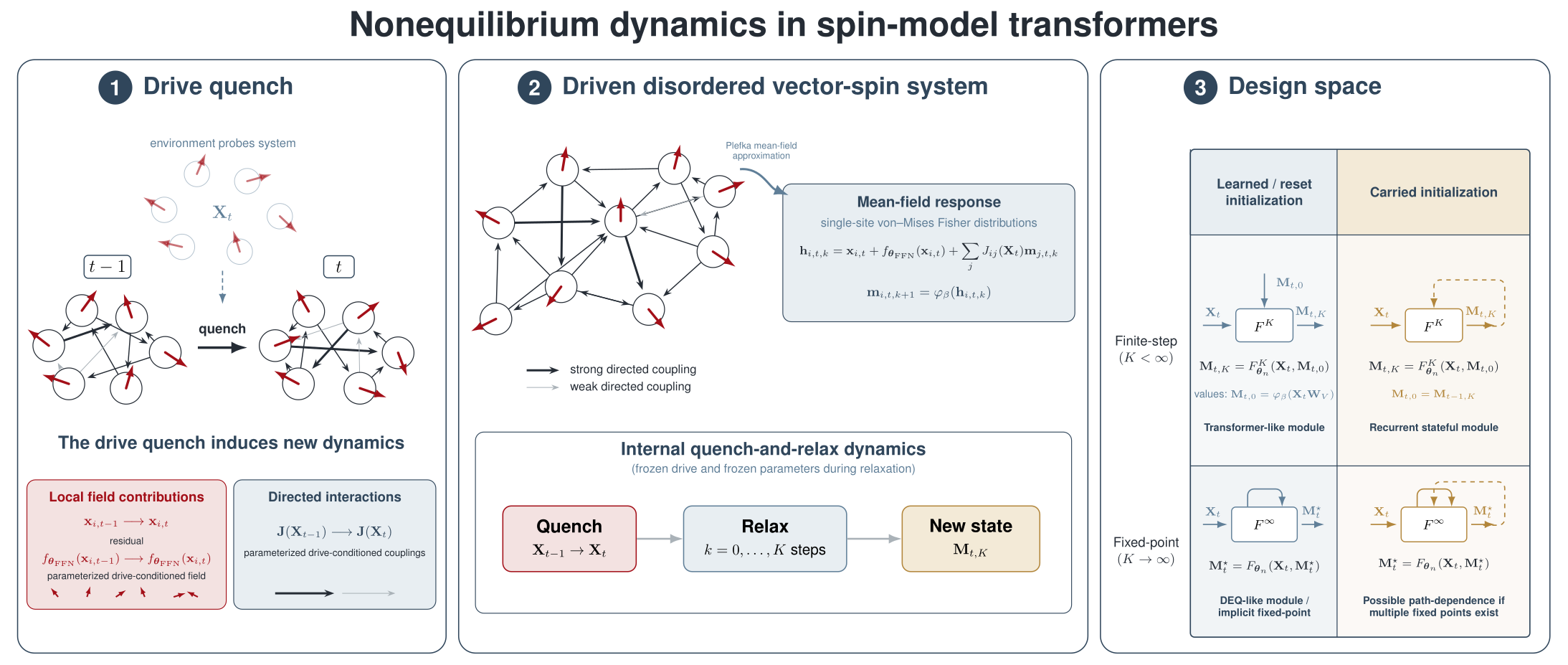
The practical value of this correspondence is that it turns transformer-shaped architectures into accelerator-friendly laboratories for driven many-body dynamics with structured, learnable couplings. Their mean-field observables must first be calibrated against exact stochastic systems at small scale, but the architectural mapping provides an interesting route to controlled experiments beyond analytically tractable toy models.
Steady-state circulation and post-quench mismatch
In this section, we show how the quench-and-relax process behind the forward pass of a spin-model transformer module relates to notions of irreversibility. We provide just5 enough physical context to introduce and motivate differentiable proxies for housekeeping entropy production6 and post-quench relaxation mismatch, both of which we can compute at the same mean-field level as the spin-model dynamics.
Quench-and-relax protocol
During relaxation after a quench we hold the input drive $\mathbf{X}_{t}$ fixed and let the spin system settle. The average magnetizations $\mathbf{M}_{t}$ may stop changing, but the system’s microscopic dynamics need not become reversible. Indeed, asymmetric couplings can sustain circulating probability currents when forward sequences of spin configurations remain more likely than their backward step reversals. We call this source of irreversibility steady-state irreversibility. Its entropy-production rate is the running cost of maintaining a nonequilibrium steady state under the current input drive. For our system, we can estimate this “housekeeping” entropy production from asymmetric couplings and delayed correlations (a vector-spin generalization of Aguilera et al., 2020),
\begin{equation} \sigma^{\star}_{\mathrm{hk},t} = \beta \sum_{ij} \left(J_{ij}(\mathbf{X}_{t}) - J_{ji}(\mathbf{X}_{t})\right) D^{\star}_{ij,t} , \label{eq:sigma_hk} \end{equation}where $D^{\star}_{ij,t}$ denote the one-step delayed correlations evaluated under the stationary one-step joint law. Intuitively, this is like
\begin{equation} \sigma^{\star}_{\mathrm{hk},t} = \sum_{ij} \left[\operatorname{directionality}\right]_{ij} \times \left[\operatorname{delayed\ flow}\right]_{ij,t}. \end{equation}The couplings provide a directional bias; the delayed correlations report whether fluctuations actually propagate along that direction.
Now we quench again. After changing the input drive abruptly, $\mathbf{X}_{t} \to \mathbf{X}_{t+1}$, the system is still distributed approximately according to its old steady state $\pi_{t}$, while the new transition rule $P_{\boldsymbol{\theta}, \mathbf{X}_{t+1}}(\mathbf{s}_{t+1, k+1} | \mathbf{s}_{t+1, k})$ induced by the new input drive actually favors another steady state $\pi_{t+1}$. The relative-entropy distance to the new frozen-drive steady state
\begin{equation} \Delta_{t+1, k} = D_{\mathrm{KL}}\left(p_{t+1,k} \lVert \pi_{t+1} \right),\label{eq:vmfkl} \end{equation}measures how far the current distribution remains from the stationary distribution selected by the new frozen drive. The new housekeeping part remains after relaxation while $\Delta_{t+1, k} \to 0$ as the actual distribution relaxes to the new stationary distribution. At the exact Markov-process level, its decrease under a fixed transition rule is associated with nonadiabatic entropy production. Below, we replace both distributions by factorized mean-field approximations and use the resulting KL-divergence as a diagnostic of post-quench lag.
A driven spin-model transformer module with asymmetric couplings can thus be diagnosed approximately in two complementary ways during the quench-and-relax process: the cost of “running” a nonequilibrium steady state after relaxation and the “catching up” during relaxation after its input drive has changed. Housekeeping entropy production measures sustained asymmetric circulation under a fixed drive while mismatch measures the relaxation still required after a drive change.
A heuristic entropy-budget interpretation: Intuitively (at the level of the exact dynamics, not necessarily at the mean-field level), every quench-and-relax cycle has an “entropy budget”
\begin{equation} \Sigma_{\mathrm{cycle}} \approx \sum^{K}_{k=1} \sigma_{\mathrm{tot},t,k} = \underbrace{\sum^{K}_{k=1} \sigma_{\mathrm{hk},t,k}}_{\text{rent, transient rate}} + \underbrace{\left( \Delta_{t,0} - \Delta_{t,K} \right)}_{\text{moving costs}} \end{equation}where the transient housekeeping $\sigma_{\mathrm{hk},t,k} = \sigma_{\mathrm{tot},t,k} - (\Delta_{t,k} - \Delta_{t,k+1})$. Appendix B supplies the corresponding transient delayed-correlation approximation; the simple housekeeping expression is recovered after taking the stationary limit. The neural-network modules defined in the corners of the design space of the previous section allocate this “entropy budget” differently depending on the number of internal relaxation steps. The DEQ corner ($K \to \infty$) fully pays off the “moving costs” every cycle and then just pays rent. The transformer corner ($K=1$ with learned initialization) barely pays rent and then does not relax the residual mismatch away. Additional frozen-protocol relaxation pays down the moving costs. This should not be conflated with protocol-updating recurrence, where feeding the response back through the module defines a new effective quench. With a carried state or a well-tuned learned initializer, we can potentially reduce the opening balance of the next cycle.
Mean-field proxy for housekeeping entropy production
Evaluating Eq. \eqref{eq:sigma_hk} at the mean-field level (see Appendix B), we arrive at the following mean-field proxy for the stationary housekeeping entropy production of the stochastic parent process,
\begin{equation} \sigma^{\star}_{\mathrm{hk},t} \approx \frac{\beta^2}{2} \sum_{ij} \left(J_{ij}(\mathbf{X}_{t}) - J_{ji}(\mathbf{X}_{t})\right)^2 C^{\star}_{ij,t} , \end{equation}where $C^{\star}_{ij,t} = \operatorname{Tr} \left( \Sigma^{\star}_{i,t} \Sigma^{\star}_{j,t} \right) \geq 0$ with $\Sigma_{i,t,k} = \operatorname{Cov} \left[ s_{i,t,k} \right]$ denoting the single-site covariances / susceptibilities. The latter is dominated by an $O(D)$ contribution that is angle-independent, so the proxy reflects mostly coupling magnitudes and susceptibility rather than representational geometry, which is captured in subleading $O(1)$ terms. For unconstrained couplings, the proxy measures squared coupling nonreciprocity, weighted by how strongly the fluctuation spaces of the two sites overlap. Under strict causal masking, however, pairwise nonreciprocity is largely enforced by the architecture. The proxy then behaves more like a susceptibility-weighted attention-concentration statistic rather than a measurement of learned asymmetry.
Mean-field proxy for post-quench relaxation mismatch
To evaluate Eq. \eqref{eq:vmfkl}, we use the fact that the mean-field vector-spin model machinery is built on the von Mises–Fisher distribution (see Appendix C), leading to the closed-form large-$D$ approximation to the factorized mean-field mismatch
\begin{equation}\Delta_{t,k}^{\mathrm{MF}}\approx\sum_i\left[R^2\log\frac{R^2-\lVert\mathbf m_{i,t}^{\star}\rVert^2}{R^2-\lVert\mathbf m_{i,t,k}\rVert^2}+\frac{2R^2\left(\lVert\mathbf m_{i,t}^{\star}\rVert^2-\mathbf m_{i,t,k}\cdot\mathbf m_{i,t}^{\star}\right)}{R^2-\lVert\mathbf m_{i,t}^{\star}\rVert^2}\right],\end{equation}where $\mathbf m_{i,t,k}$ is the current magnetization and $\mathbf m_{i,t}^{\star}$ is the target instantaneous fixed-point magnetization. The expression vanishes when $\mathbf m_{i,t,k}=\mathbf m_{i,t}^{\star}$ at every site and penalizes both differences in magnetization norm and angular misalignment with the frozen-drive fixed-point response.
Numerical experiments
In this section, we first delineate where the mean-field approximation can be trusted by comparing mean-field quantities to their respective sampled estimates obtained from simulations of the stochastic dynamics of the vector-spin model. We then train a toy transformer-like stack of modules to do character-level language modeling and probe and measure its behavior.
Mean-field approximation and proxy fidelity
We simulate a system of $N=64$ vector spins wobbling about on spheres of radius $R=\sqrt{D/2-1}$ towards steady state, using a dense asymmetric coupling matrix obtained by applying a row-wise softmax to Gaussian random entries7. The external fields have independent, random orientations but equal norm at every site. We stress that this quenched random realization is deliberately not representative of the kind of couplings and external fields that the system would have if it were exposed to structured data and trained as a neural-network module: it is not representative of trained systems but gives us some idea of what to expect8.
To control the overall strength of the drive, we introduce the parameter $u=\beta\lVert \mathbf{x}\rVert/R$ as a homogeneous dimensionless drive amplitude. We sweep the symmetric grid $\{0.25,0.5,0.75,1,1.5,2,4\}$ for a few values of the vector dimension $D$ to obtain steady-state “calibration maps” for the magnetizations, the one-step delayed correlations, and the housekeeping entropy production. Each heatmap cell below reports the larger of the noise-corrected relative mean-field error and its Monte Carlo sampling9 floor. Let us first compare the mean-field approximation to the exact stochastic dynamics.
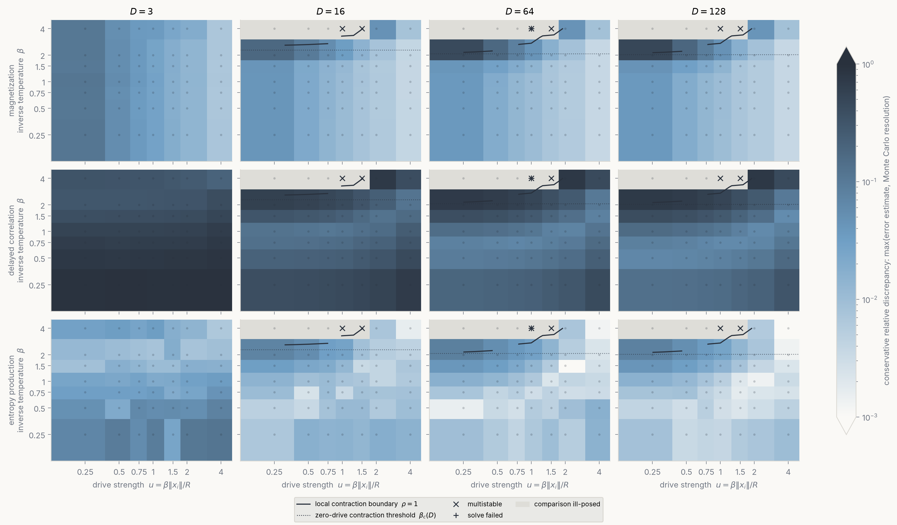
We observe that steady-state magnetizations are accurately captured, while the one-step delayed correlations show discrepancies of roughly 10% or more, as expected for a first-order Plefka[t-1,t] approximation. Yet the housekeeping entropy production is remarkably accurate, which is surprising since it is computed from the delayed correlations10. One possible explanation is that the leading approximation preserves the time-antisymmetric component selected by $J-J^{T}$, even when the full delayed-correlation matrix remains imperfect.
As expected for a high-temperature expansion, the Plefka mean-field approximation deteriorates as $\beta$ increases for fixed $u$, while stronger pinning (larger drive strength $u$) partially stabilizes it. Intuitively, this is the competition between the drive and the interactions. If the drive dominates, then we are in an easy regime and responses are pretty much aligned with the drive. If the drive is small and interactions dominate, then mean-field will start struggling. (This balancing act might be familiar to practitioners who have tuned the relative strength of residuals in neural networks.)
Let us now check the next rung in the approximation ladder and compare the mean-field quantities to their large-$D$ approximations2, which we use in practice.
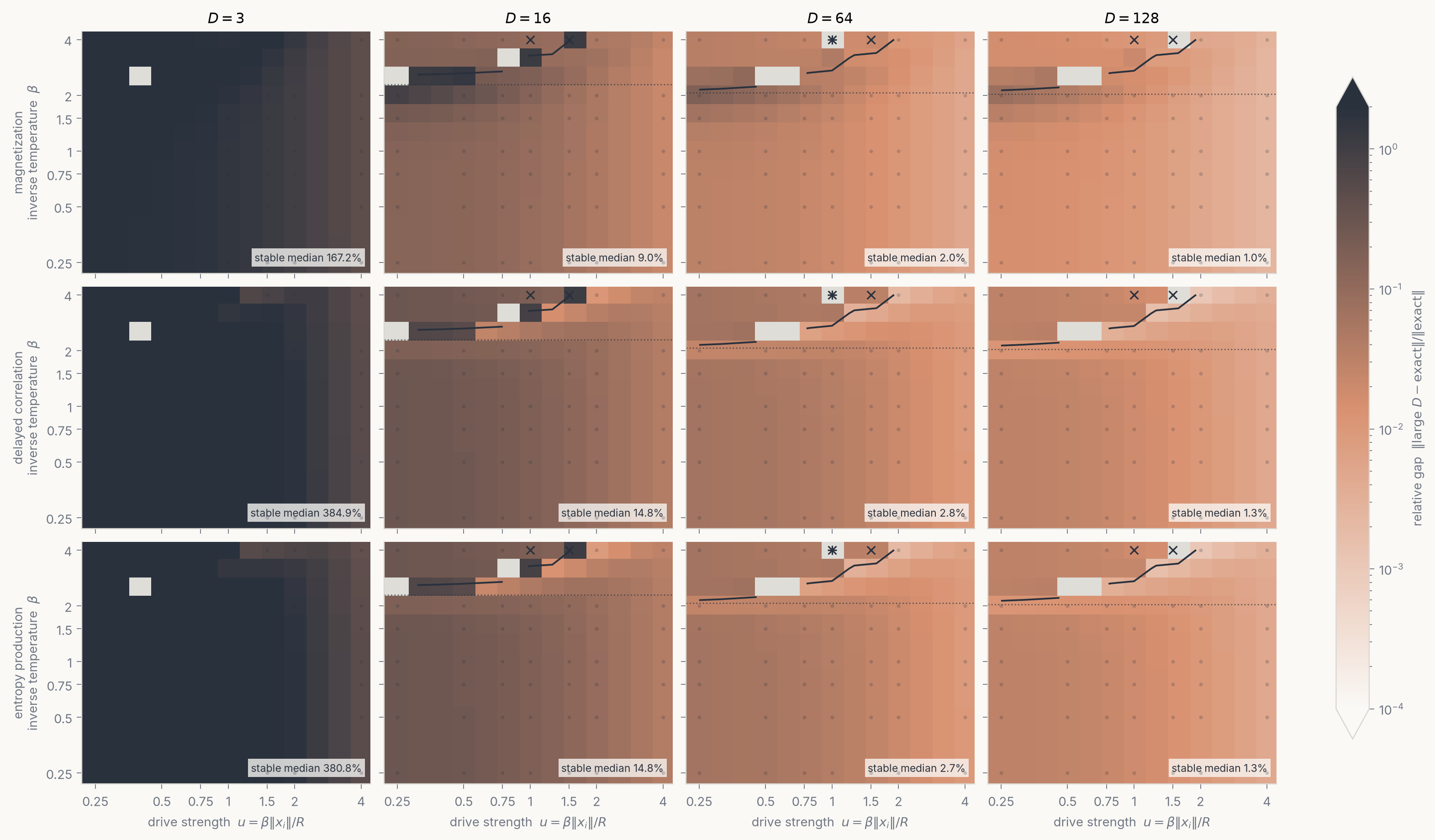
We observe that the closed-form large-$D$ approximation quickly converges to the exact finite-$D$ mean-field quantities, with errors roughly scaling as $O(1/D)$. The temporal-factorization error of the simple Plefka[t-1,t] mean-field closure persists, as expected. Near the operating regime $(u,\beta)=(1,1)$, the delayed-correlation discrepancy converges to approximately 11%, while magnetization remains accurate at the percent level.
Training a toy autoregressive language model
Having calibrated the approximation stack in a controlled random system, let us now take a leap and immediately test the deterministic mean-field module in a structured training environment. Let us train small autoregressive language models to do character-level next-token prediction on The Brothers Karamazov. This exercise should feel very familiar, and that is exactly the point: if we claim that the transformer-like architecture in the design space (one-step update + learned initializer) looks pretty much like a parallel transformer block, it also better behave like one in real training scenarios.
The architecture
We build a simple autoregressive language model by stacking causal finite-step modules with a final map from final-layer magnetizations to logits:
class LanguageModel(nn.Module):
    def __init__(
        self,
        vocab: int,
        dim: int,
        depth: int,
        heads: int,
    ):
        super().__init__()
        self.embedding = nn.Embedding(vocab, dim)
        self.layers = nn.ModuleList(
            SpinModelTransformerModule(
                dim=dim,
                num_heads=heads,
                num_steps=1,        # K=1 (finite-step relaxation, no steady state)
                init="learned",     # learned initializer (~ values)
                input_mode="field" if layer_index == 0 else "magnetization",
                beta=1.0,
                causal=True,
                rope=True,
            )
            for layer_index in range(depth)
        )
        self.to_logits = nn.Sequential(nn.RMSNorm(dim), nn.Linear(dim, vocab, bias=False))
        # make sure the initial embeddings are sensibly scaled
        with torch.no_grad():
            vectors = self.embedding.weight.view(vocab, heads, dim // heads)
            vectors.copy_(self.layers[0].radius_head * F.normalize(vectors, dim=-1))

    def forward(self, token_ids: Tensor):
        x = self.embedding(token_ids)
        for layer in self.layers:
            x = layer(x).magnetizations
        return self.to_logits(x)
On stability and depth
A salient implementation detail is the module’s input_mode, which is related to pre-norm normalization conventions in transformers and the stability of the forward and backward passes. We treat token embeddings presented to the first layer as physical fields added as residuals to the update step. In subsequent layers, the inputs are instead treated as conjugate fields of the magnetizations of the previous layer. Why do we do this? Because the residual stream is a shared communication bus, and we should try to keep it open and flowing. If we decided to pass magnetizations between modules like $\mathbf{m}_{\mathrm{out}} = \varphi_{\beta} \left( \mathbf{m}_{in} + \Delta_{\mathbf{h}} \right)$, then the contractiveness of the response map $\varphi_{\beta}$ would attenuate both signals and gradients with depth, even for $\Delta_{\mathbf{h}}=\mathbf{0}$. If we instead propagate signal like $\mathbf{m}_{\mathrm{out}} = \varphi_{\beta} ( \varphi^{-1}_{\beta} (\mathbf{m}_{in}) + \Delta_{\mathbf{h}} )$ then $\mathbf{m}_{\mathrm{out}} = \mathbf{m}_{in}$ for $\Delta_{\mathbf{h}}=\mathbf{0}$, where $\varphi^{-1}_{\beta} (\mathbf{m}_{in})$ denotes the conjugate field required to sustain $\mathbf{m}_{in}$. Luckily, for the large-$D$ response, the inverse map of Eq. \eqref{eq:paralleltransformer} is analytic inside the open magnetization ball:
The loss goes down…
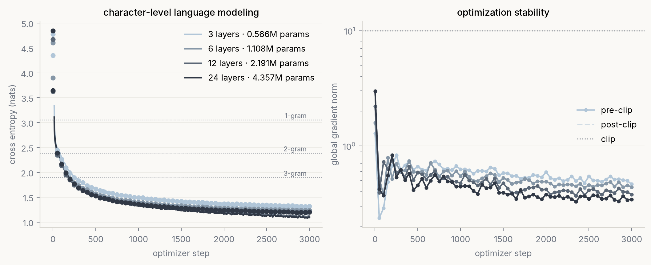
We trained 3-, 6-, 12-, and 24-layer versions11 of the model with seq_len=128, dim=128, num_heads=4, and dim_head=32, and observed smooth, stable convergence.
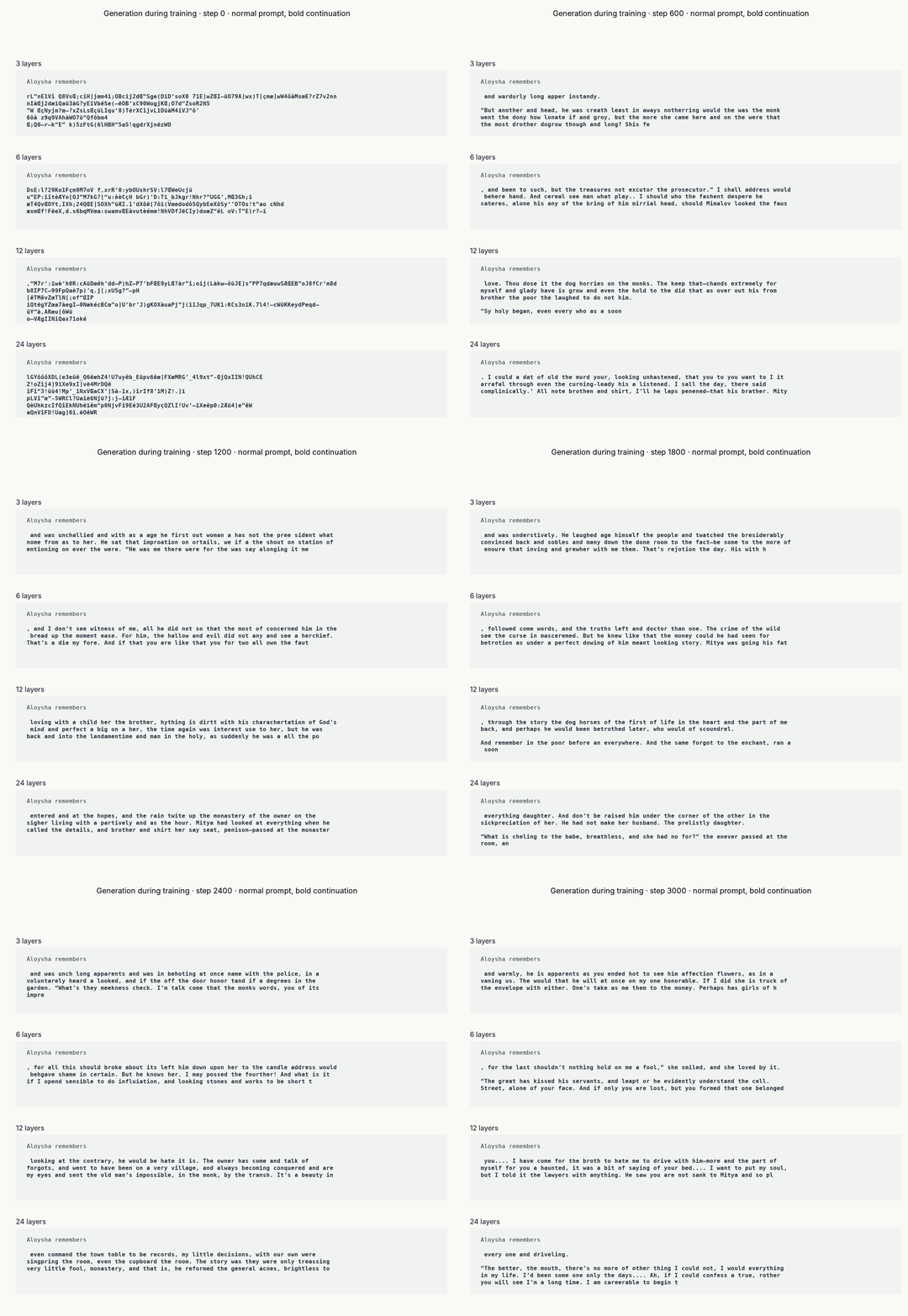
During training, we generated fixed-seed top-k samples. Alyosha remembers love.
… but do the modules behave?
We checked the competition between terms in the update equation after training. Feed-forward and attention terms remain competitive, and the residual grows with depth like in pre-norm transformers.
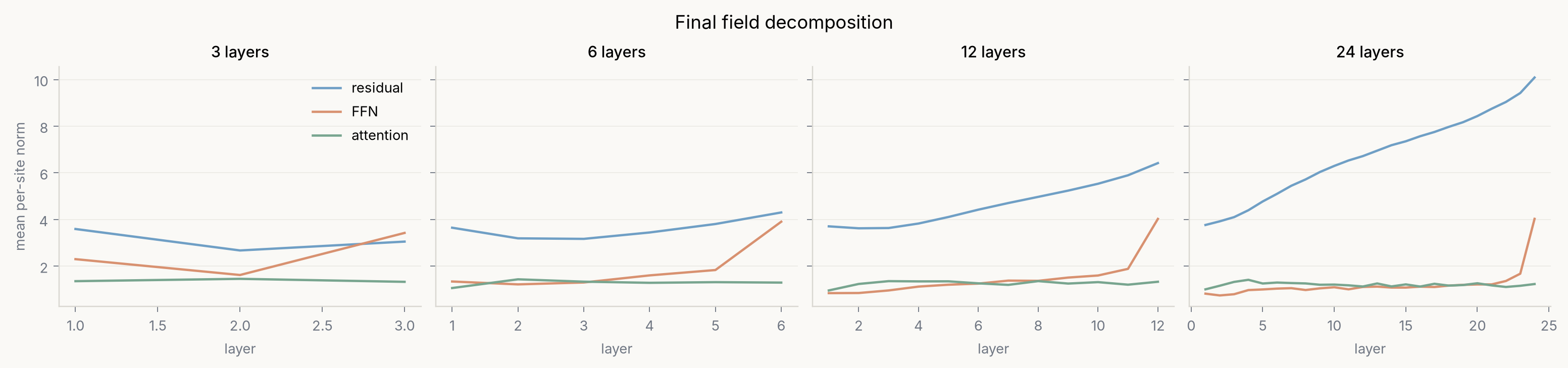
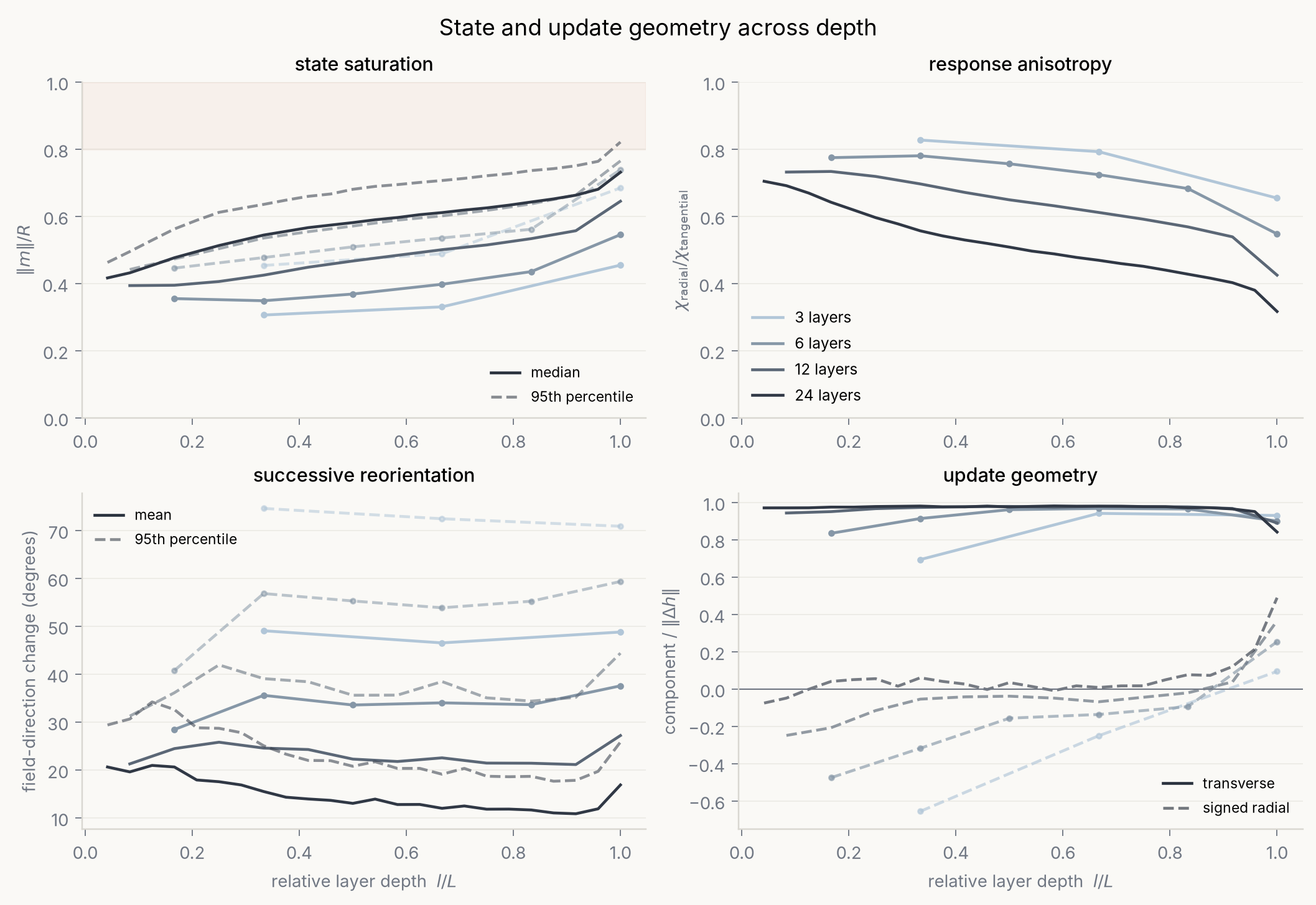
This residual-norm growth is not felt by the feed-forward and attention terms since they see normalized inputs. Recall from the stability-and-depth paragraph above that these growing residuals are effective fields $\mathbf{h}$ associated with bounded magnetizations $\mathbf{m} = \varphi_{\beta} \left(\mathbf{h}\right)$ whose norms never exceed $R$. These could saturate, but we did not observe that during these runs. We also verified that later layers continued to produce substantial directional updates before the logits readout.
Measuring the frozen-drive steady-state irreversibility proxy
To demonstrate proxy instrumentation, we also logged the evolution of average frozen-drive steady-state irreversibility associated with the instantaneous steady-state fixed points for every layer. We observe that the proxy gradually rises and stabilizes during training after an initial drop. Recall from earlier that, under causal masking, pairwise nonreciprocity is largely enforced by the architecture, so the proxy measures susceptibility-weighted attention-concentration rather than learned asymmetry.
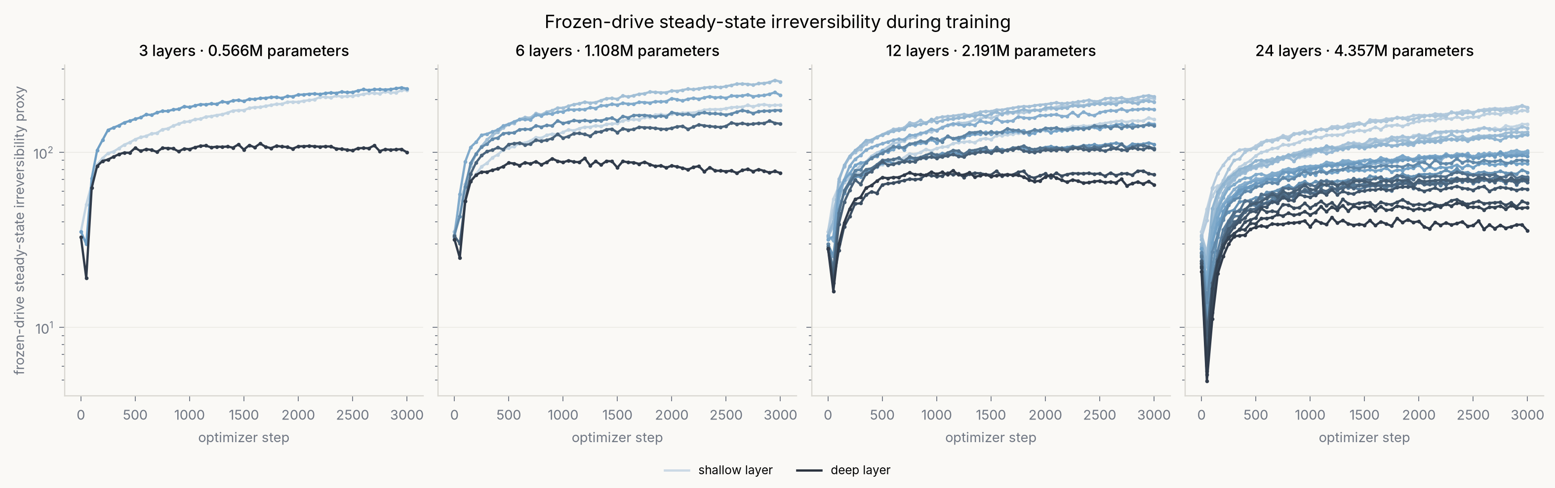
This experiment demonstrates that the frozen-drive irreversibility proxy can be measured throughout training. Notably, the steady-state irreversibility above is measured at the hypothetical continuation of each layer towards its frozen-drive fixed point. Away from stationarity, the steady-state cancellation used to derive the housekeeping entropy production formula Eq. \eqref{eq:sigma_hk} no longer holds and things get considerably more complicated. Even though the modules never visit their fixed points when run at $K=1$, there might still be a relation because the same update equation determines both the first step and the eventual frozen-drive steady state.
So the instrumentation is available, but the more basic question is whether training has any incentive to approach these frozen-drive fixed points at all.
Training at $K=1$ selects a nonequilibrium transient
Let us focus on the 6-layer model and test the end-to-end loss effect when increasing $K$ to 2, 4, and $\infty$ for layer $\ell$ at inference time. This intervention measures the network’s sensitivity to moving layer $\ell$ farther along its local relaxation path, including how downstream layers respond to that now-slightly-off-distribution representation.
In a one-layer-at-a-time intervention, the manipulated layer $\ell$ follows its original frozen-protocol relaxation trajectory because its incoming representation is unchanged. Its altered output nevertheless changes the drives and couplings of all subsequent layers, so the resulting loss penalty should be understood as an end-to-end downstream response rather than a strictly local effect. The joint intervention compounds such direct relaxation changes throughout the stack. Only the final-layer intervention is most directly interpretable with respect to the task loss, since there are no subsequent spin-model layers whose protocols are changed.
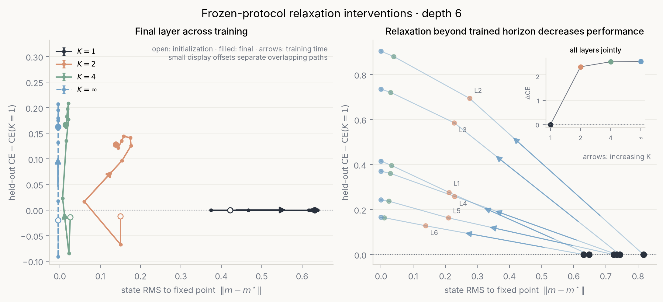
In all cases, we find that additional internal relaxation does not guarantee convergence toward a better answer: the $K=1$ finite-step module outputs are not underconverged approximations of their respective layers’ fixed points. Since the model was trained at $K=1$, it is perhaps not surprising that relaxing for more iterations at inference time can hurt performance, even though each layer intervention lies along that layer’s well-defined frozen-protocol relaxation trajectory. But there is an interesting hypothesis here provided by the spin-model framework: maybe training at finite $K$ makes use of nonequilibrium transient states. Since relaxation horizon is an architectural control, a module trained at $K=1$ can specialize its computation to the finite-time state rather than trying to reach a fixed point that is perhaps not where it needs to go.
To poke at this hypothesis, let us focus on the learned values at $K=1$, which are initializer states for the update equation. We intervene on one layer at a time while leaving the parameters and update rules of all other layers unchanged. As before in the relaxation interventions, the altered outputs nevertheless change the drives and couplings encountered downstream. We replace the learned values with controls like the residual, all-zeros, or shuffled values. Across layers, we find that the learned values are tuned for task-relevant one-step transitions, not for fixed-point proximity.
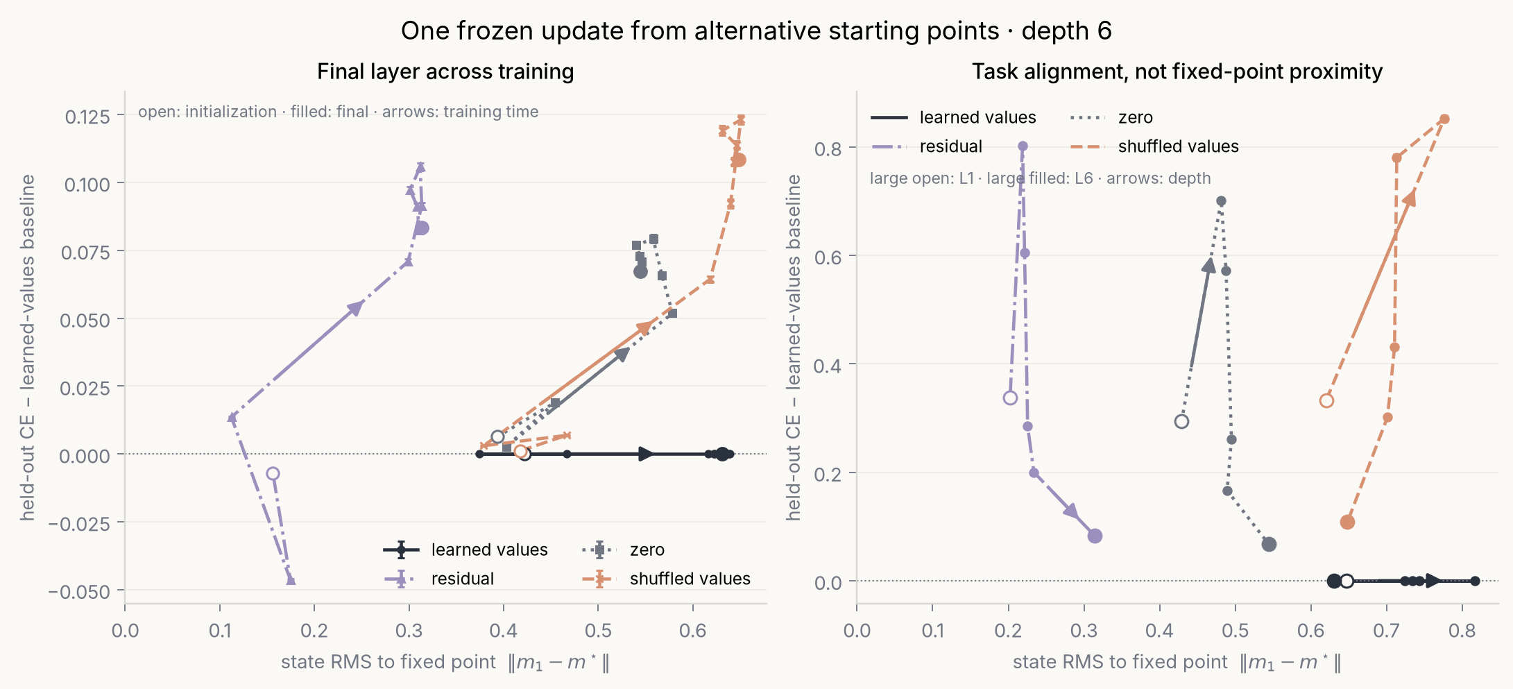
Again, a trained initializer working better than untrained substitutes is expected. But the suggestive pieces of information are that (1) starting from the residual lands much closer to the fixed point after one step, yet performs worse, (2) learned values remain farther from the fixed point, yet give the best task result, and (3) shuffled values approximately preserve the distance to the fixed point but break its alignment with the current drive and routing so performance decreases. Intuitively, learned values amortize the search for a good one-step task-relevant starting state from inputs, across the dataset. Fixed-point proximity is not an implicit objective, and useful computation can be found in the transient.
Conclusion and outlook
In this post, we have further refined the connection between mean-field vector-spin models and transformer-like neural networks as introduced in Deep Implicit Attention: A Mean-Field Theory Perspective on Attention Mechanisms (2021). We have shown how to build neural-network modules around a quench-and-relax protocol applied to simple mean-field approximations of driven nonequilibrium asymmetric vector-spin systems. We also discussed two measurable aspects of their dynamics: steady-state circulation under a fixed drive and post-quench relaxation following a change in the drive. Numerical experiments suggest that learning in these systems can exploit controlled nonequilibrium transients rather than approximate fixed-point computation.
It would be interesting to consider the possible prediction, clamping, and parameter-update protocols that could be built around these dynamics, including temporal Hebbian-like learning rules. Do the proxies we introduced reveal anything useful about how such systems learn or adapt under changing drives? Can we use mismatch proxies as a halting signal for adaptive test-time compute? To what other architectures do less simple mean-field approximations lead? Do useful models always rely on transient states and finite-step relaxation? What changes when state is carried between quenches or modules drive one another?
References
If you happen to find this work useful, please consider citing it as:
@article{bal2026neqnn,
  title   = {Nonequilibrium Dynamics in Spin-Model Transformers},
  author  = {Bal, Matthias},
  year    = {2026},
  month   = {August},
  url     = {https://mcbal.github.io/post/nonequilibrium-dynamics-in-spin-model-transformers/}
}
Relevant literature: stochastic thermodynamics of driven steady states; dynamical mean-field theory for asymmetric spin systems; recurrent-depth and implicit neural computation; prediction, physical learning, and driven adaptation
A non-exhaustive list of references and inspiration includes:
- A unifying framework for mean-field theories of asymmetric kinetic Ising systems (2020) by Miguel Aguilera, S. Amin Moosavi, and Hideaki Shimazaki
- Deep Equilibrium Models (2019) by Shaojie Bai, J. Zico Kolter, and Vladlen Koltun
- Three detailed fluctuation theorems (2009) by Massimiliano Esposito and Christian Van den Broeck
- Self-organized fine-tuned response in a driven spin glass (2021) by Jacob Mitchell Gold
- The thermodynamics of prediction (2012) by Susanne Still, David A. Sivak, Anthony J. Bell, and Gavin E. Crooks
Appendices
Appendix A: Symbol glossary
| Symbol | Meaning |
|---|---|
| State & geometry | |
| $\mathbf{s}_{i,t,k}\in\mathbb{R}^D$ | Vector spin at site $i$, external time $t$, relaxation step $k$ |
| $\mathbf{m}_{i,t,k}$ | Magnetization (spin expectation value) at relaxation step $k$ |
| $\mathbf{h}_{i,t,k}$ | Effective field acting on site $i$ |
| $N, D$ | Number of sites (spins); vector-spin dimension |
| $R^2=D/2-1$ | Spin-sphere radius (large-$D$ approximation) |
| $\beta$ | Inverse temperature |
| Drive & coupling | |
| $\mathbf{x}_{i,t}$ | Local external field / drive at site $i$ |
| $\mathbf{X}_t\in\mathbb{R}^{N\times D}$ | Full drive / context window at step $t$ |
| $J_{ij}(\mathbf{X}_t)$ | Drive-conditioned coupling (softmax attention) |
| $f_{\theta_{\text{FFN}}}$ | Position-wise drive-conditioned field (FFN-like) |
| $\varphi_\beta$ | Magnetization response map (Eq. \eqref{eq:paralleltransformer}) |
| $\varphi_\beta^{-1}$ | Conjugate-field inverse of $\varphi_\beta$ |
| Clocks | |
| $k$ | Fast internal relaxation index |
| $t$ | Drive / input-context index (quench clock) |
| $n$ | Slow parameter-update index (learning clock) |
| $\ell$ | Layer / depth index |
| $K$ | Relaxation horizon (# internal steps before next quench) |
| $\theta,\eta$ | Parameters; learning rate |
| Irreversibility & mismatch | |
| $\pi_t$ | Frozen-drive nonequilibrium steady state (NESS) |
| $\mathbf{M}^\star_t$ | Fixed-point magnetizations under frozen drive $X_t$ |
| $\sigma^\star_{\mathrm{hk},t}$ | Housekeeping entropy-production rate |
| $D^\star_{ij,t}$ | Stationary one-step delayed correlation |
| $\Delta_{t,k}$ | Post-quench relaxation mismatch (KL to $\pi_t$) |
| $\Sigma_{i,t,k}$ | Single-site covariance / susceptibility |
| $\rho_t=\beta J_t/2$ | Contractiveness ratio (stability of $\varphi_\beta$) |
Appendix B: Mean-field delayed correlations and housekeeping entropy production
To evaluate Eq. \eqref{eq:sigma_hk}, we need stationary one-step delayed correlations $D^{\star}_{ij,t}$. To this end, let us first compute a first-order Plefka[t-1,t] mean-field approximation of the transient one-step delayed correlations $D_{ij,t,k}$,
Evaluating this expression as we did for the magnetizations in Spin-Model Transformers (2023), we end up with the mean-field approximation
\begin{align} D_{ij,t,k} \approx \beta J_{ij}(\mathbf{X}_{t}) \operatorname{Tr} \left( \Sigma_{i,t,k} \Sigma_{j,t,k-1} \right), \end{align}where $\Sigma_{i,t,k} = \operatorname{Cov} \left[ s_{i,t,k} \right]$ denotes the single-site covariance / susceptibility. The trace captures which directions on the vector-spin sphere are still available to fluctuate. If a spin is weakly magnetized, it has many soft directions. If it is strongly magnetized, many directions are suppressed because the spin is pinned close to its mean direction.
At stationarity, $p_{t,k-1} \to \pi_{t}$ and $\mathbf{m}_{i,t,k} \to \mathbf{m}^{\star}_{i,t}$ so that
\begin{align} D^{\star}_{ij,t} = \lim_{k\to\infty} D_{ij,t,k} = \mathbb{E}_{\mathbf{s} \sim \pi_{t}, \mathbf{s'} \sim P_{\boldsymbol{\theta}, \mathbf{X}_{t}}(\cdot | \mathbf{s})} \left[ \left( \mathbf{s'}_{i} - \mathbf{m}^{\star}_{i,t} \right) \cdot \left( \mathbf{s}_{j} - \mathbf{m}^{\star}_{j,t}\right) \right] \end{align}and the mean-field approximation becomes
\begin{align} D^{\star}_{ij,t} \approx \beta J_{ij}(\mathbf{X}_{t}) \operatorname{Tr} \left( \Sigma^{\star}_{i,t} \Sigma^{\star}_{j,t} \right), \end{align}Substituting the large-$D$ approximation from Spin-Model Transformers (2023),
\begin{align} \Sigma_{i,t} \approx \frac{\mathbf{I}_{D}}{1+\gamma_{i,t}} - \frac{\mathbf{m}_{i,t} \mathbf{m}_{i,t}^{T}}{R^2 \gamma_{i,t}}, \end{align}we end up with the $(i \leftrightarrow j)$-symmetric explicit expression
\begin{align} C^{\star}_{ij,t} &= \operatorname{Tr} \left( \Sigma^{\star}_{i,t} \Sigma^{\star}_{j,t} \right) \geq 0 \nonumber \\ &= \frac{D}{(1+\gamma^{\star}_{i,t})(1+\gamma^{\star}_{j,t})} \nonumber\\ &- \frac{\lVert \mathbf{m}^{\star}_{j,t} \rVert^2}{R^2 \gamma^{\star}_{j,t} \left( 1 + \gamma^{\star}_{i,t} \right)} \nonumber\\ &- \frac{\lVert \mathbf{m}^{\star}_{i,t} \rVert^2}{R^2 \gamma^{\star}_{i,t} \left( 1 + \gamma^{\star}_{j,t} \right)} \nonumber\\ &+ \frac{\left( \mathbf{m}^{\star}_{i,t} \cdot \mathbf{m}^{\star}_{j,t} \right)^2}{R^4 \gamma^{\star}_{i,t} \gamma^{\star}_{j,t}}, \end{align}where
\begin{align} \gamma^{\star}_{i,t} &= \sqrt{1 + \beta^2 \lVert \mathbf{h}^{\star}_{i,t} \rVert^2 / R^2 },\\ \mathbf{h}^{\star}_{i,t} &= \mathbf{x}_{i,t} + f_{\theta_{\text{FFN}}} \left( \mathbf{x}_{i,t} \right) + \sum_{l} J_{il} (\mathbf{X}_{t}) \mathbf{m}^{\star}_{l,t}. \end{align}Since $\gamma^{\star} \sim O(1)$, the one-step delayed correlations $D^{\star}_{ij,t}$ are dominated by a large angle-independent isotropic contribution $O(D)$ with the other three terms being $O(1)$. The housekeeping entropy production proxy in the Plefka[t-1,t] approximation becomes
or, using the symmetry of $C^{\star}_{ij,t}$,
\begin{equation} \sigma^{\star}_{\mathrm{hk},t} \approx \frac{\beta^2}{2} \sum_{ij} \left(J_{ij}(\mathbf{X}_{t}) - J_{ji}(\mathbf{X}_{t})\right)^2 C^{\star}_{ij,t} . \end{equation}Appendix C: The von Mises–Fisher distribution: Kullback-Leibler divergence
The natural distribution for a directional variable $\mathbf u$ on the unit hypersphere $S^{D-1}$ is the von Mises–Fisher distribution,
\begin{equation}q(\mathbf u\mid\boldsymbol\mu,\kappa)=C_D(\kappa)\exp\left(\kappa\boldsymbol\mu^\top\mathbf u\right),\end{equation}where $\boldsymbol\mu$ is a unit vector giving the mean direction and $\kappa\geq 0$ is the concentration. For two such distributions $q_a=q(\boldsymbol\mu_a,\kappa_a)$ and $q_b=q(\boldsymbol\mu_b,\kappa_b)$, the KL divergence is
\begin{equation}D_{\mathrm{KL}}(q_a\Vert q_b)=\log\frac{C_D(\kappa_a)}{C_D(\kappa_b)}+A_D(\kappa_a)\left(\kappa_a-\kappa_b\boldsymbol\mu_a^\top\boldsymbol\mu_b\right),\end{equation}with
\begin{equation}A_D(\kappa)=\frac{I_{D/2}(\kappa)}{I_{D/2-1}(\kappa)}.\end{equation}The divergence therefore measures both a mismatch in concentration and a mismatch in direction.
In the vector-spin model, the spins have fixed radius $R$, so we write $\mathbf s=R\mathbf u$. The single-site conditional distribution under an effective field $\mathbf h$ is
\begin{equation}q(\mathbf s\mid\mathbf h)\propto\exp\left(\beta\mathbf h \cdot \mathbf s\right)=\exp\left(\beta R\lVert\mathbf h\rVert \times \left(\frac{\mathbf h}{\lVert\mathbf h\rVert} \cdot \mathbf u\right)\right).\end{equation}Its vMF parameters are therefore
\begin{equation}\boldsymbol\mu_{\mathbf h}=\frac{\mathbf h}{\lVert\mathbf h\rVert},\qquad \kappa_{\mathbf h}=\beta R\lVert\mathbf h\rVert.\end{equation}Thus $\boldsymbol\mu$ is not the effective field itself, but its normalized direction. Likewise, the concentration is not generally $\beta$: it combines inverse temperature, spin radius, and field magnitude. Only in the special case $R=1$ and $\lVert\mathbf h\rVert=1$ do we obtain $\boldsymbol\mu=\mathbf h$ and $\kappa=\beta$. The corresponding mean magnetization is
\begin{equation}\mathbf m(\mathbf h)=R A_D(\kappa_{\mathbf h})\boldsymbol\mu_{\mathbf h}.\end{equation}For the spin-model transformer module, the effective field at site $i$, external step $t$, and internal relaxation step $k$ is
\begin{equation}\mathbf{h}_{i,t,k} = \mathbf{x}_{i,t} + f_{\boldsymbol{\theta}_{\mathrm{FFN}}}\left( \mathbf{x}_{i,t} \right) + \sum_{j} J_{ij} (\mathbf{X}_{t}) \mathbf{m}_{j,t,k}.\end{equation}Each mean-field state therefore defines a factorized vMF approximation,
\begin{equation}q_{t,k}(\mathbf s)=\prod_i q\left(\mathbf s_i\mid\boldsymbol\mu_{i,t,k},\kappa_{i,t,k}\right),\end{equation}with
\begin{equation}\boldsymbol\mu_{i,t,k}=\frac{\mathbf h_{i,t,k}}{\lVert\mathbf h_{i,t,k}\rVert},\qquad \kappa_{i,t,k}=\beta R\lVert\mathbf h_{i,t,k}\rVert.\end{equation}If $q_t^\star$ denotes the corresponding frozen-drive fixed-point distribution, the post-quench mean-field mismatch can be monitored through
\begin{equation}\Delta_{t,k}^{\mathrm{MF}}=D_{\mathrm{KL}}\left(q_{t,k}\Vert q_t^\star\right)=\sum_i D_{\mathrm{KL}}\left(q_{i,t,k}\Vert q_{i,t}^\star\right).\end{equation}This quantity compares the system’s current directional and concentration state with the stationary mean-field response associated with the current drive. It approaches zero as the mean-field state relaxes to that fixed point. In the zero-field case, $\kappa=0$ and the vMF distribution is uniform, so its mean direction is irrelevant.
Explicitly, the single-site contribution comparing the current state $q_{i,t,k}$ with the frozen-drive fixed-point state $q_{i,t}^{\star}$ is given by
\begin{equation}D_{\mathrm{KL}}\left(q_{i,t,k}\Vert q_{i,t}^{\star}\right)=\log\frac{C_D(\kappa_{i,t,k})}{C_D(\kappa_{i,t}^{\star})}+A_D(\kappa_{i,t,k})\left(\kappa_{i,t,k}-\kappa_{i,t}^{\star}\boldsymbol\mu_{i,t,k}\cdot\boldsymbol\mu_{i,t}^{\star}\right).\end{equation}Substituting $\boldsymbol\mu_{\mathbf h}=\mathbf h/\lVert\mathbf h\rVert$ and $\kappa_{\mathbf h}=\beta R\lVert\mathbf h\rVert$ gives the equivalent effective-field expression
\begin{equation}D_{\mathrm{KL}}\left(q_{\mathbf h_a}\Vert q_{\mathbf h_b}\right)=\log\frac{C_D(\beta R\lVert\mathbf h_a\rVert)}{C_D(\beta R\lVert\mathbf h_b\rVert)}+\beta R A_D(\beta R\lVert\mathbf h_a\rVert)\left(\lVert\mathbf h_a\rVert-\frac{\mathbf h_a\cdot\mathbf h_b}{\lVert\mathbf h_a\rVert}\right).\end{equation}Here $\mathbf h_a$ parameterizes the distribution in the first argument of the KL divergence and $\mathbf h_b$ parameterizes the reference distribution in the second argument. The original vMF form above remains well defined when $\mathbf h_a=\mathbf 0$, in which case $\kappa_a=0$ and its mean direction is irrelevant.
In the large-vector-dimension limit, we again set $R^2=D/2-1$ and introduce
\begin{equation}\gamma_{\mathbf h}=\sqrt{1+\frac{\beta^2\lVert\mathbf h\rVert^2}{R^2}}.\end{equation}Using the leading large-$D$ magnetization response $\mathbf m_{\mathbf h}\approx\beta\mathbf h/(1+\gamma_{\mathbf h})$, the KL divergence becomes
\begin{equation}D_{\mathrm{KL}}^{D\to\infty}\left(q_{\mathbf h_a}\Vert q_{\mathbf h_b}\right)\approx\frac{\beta^2\left(\lVert\mathbf h_a\rVert^2-\mathbf h_a\cdot\mathbf h_b\right)}{1+\gamma_{\mathbf h_a}}+R^2\left(\gamma_{\mathbf h_b}-\gamma_{\mathbf h_a}-\log\frac{1+\gamma_{\mathbf h_b}}{1+\gamma_{\mathbf h_a}}\right).\end{equation}The same expression can be written entirely in terms of the corresponding magnetizations. The large-$D$ response can be inverted as
\begin{equation} \mathbf{h}\approx\frac{2R^2}{\beta\left(R^2-\lVert\mathbf{m}\rVert^2\right)}\mathbf{m},\qquad \lVert\mathbf{m}\rVert < R. \end{equation}Substitution gives the magnetization-only form
\begin{equation}D_{\mathrm{KL}}^{D\to\infty}\left(q_{\mathbf m_a}\Vert q_{\mathbf m_b}\right)\approx R^2\log\frac{R^2-\lVert\mathbf m_b\rVert^2}{R^2-\lVert\mathbf m_a\rVert^2}+\frac{2R^2\left(\lVert\mathbf m_b\rVert^2-\mathbf m_a\cdot\mathbf m_b\right)}{R^2-\lVert\mathbf m_b\rVert^2}.\end{equation}For the post-quench relaxation considered here, $\mathbf m_a=\mathbf m_{i,t,k}$ is the current magnetization and $\mathbf m_b=\mathbf m_{i,t}^{\star}$ is the instantaneous fixed-point magnetization. The corresponding large-$D$ factorized mismatch is therefore
\begin{equation}\Delta_{t,k}^{\mathrm{MF}}\approx\sum_i\left[R^2\log\frac{R^2-\lVert\mathbf m_{i,t}^{\star}\rVert^2}{R^2-\lVert\mathbf m_{i,t,k}\rVert^2}+\frac{2R^2\left(\lVert\mathbf m_{i,t}^{\star}\rVert^2-\mathbf m_{i,t,k}\cdot\mathbf m_{i,t}^{\star}\right)}{R^2-\lVert\mathbf m_{i,t}^{\star}\rVert^2}\right].\end{equation}This expression is asymmetric, as required for a KL divergence. It vanishes when $\mathbf m_{i,t,k}=\mathbf m_{i,t}^{\star}$ at every site and penalizes both differences in magnetization norm and angular misalignment with the frozen-drive fixed-point response.
Footnotes
A first-order expansion around the non-interacting system between consecutive (internal relaxation) time slices. See Spin-Model Transformers (2023). ↩︎
The large-$D$ approximation avoids repeated evaluation of modified Bessel functions originating from the von Mises–Fisher distribution used in the ansatz for the decoupled mean magnetizations. It is mainly motivated by the empirical fact that the embedding dimensions in modern neural networks are large. See Spin-Model Transformers (2023) for full details. ↩︎ ↩︎
A drive-dependent coupling rule turns a fixed-size $N \times N$ coupling matrix into a parameterized rule that supports variable system size, drive-conditioned routing, and a way to scale system size without learning new explicit parameters. Softmax attention is a convenient choice for a bounded positive row-stochastic coupling rule. Other possible choices include additive or multiplicative combinations with slower base coupling parameters $\mathbf{J}^{0}$ that are drive-independent, leading to a system with persistent interactions in the absence of a drive. ↩︎
In this case, it is more accurate to call the drive $\mathbf{X}_{t}$ an external protocol parameter configuring the instantaneous dynamics. ↩︎
We deliberately focus on our simple quench-and-relax use case because the nonequilibrium thermodynamics literature is very nuanced and, quite frankly, a daunting terminological minefield. ↩︎
We are talking about the entropy production associated with the module’s explicit stochastic parent dynamics. This is not about hardware energy consumption or physical dissipation. ↩︎
In the spirit of this post, this corresponds to one quenched coupling realization rather than a disorder-averaged result. We also fix $N$ and do not look at scaling in $N$ because (1) the control variable is really an effective $N_{\mathrm{eff}}$ determined by the concentration of the couplings, which, for our purposes, will be learned anyway and training might just ensure $N_{\mathrm{eff}} \sim O(1)$, (2) we expect that increasing effective connectivity should systematically improve one-point mean-field fidelity, while relative errors in the vanishing pairwise correlations probably will not disappear in the first-order approximation considered in this post, and (3) practical applications like causal attention have early rows with only a small number of available predecessors by construction, so their effective system size remains small even for large sequence length. ↩︎
Averaging more random realizations would establish typicality and steady-state behavior only within this artificial random ensemble. Future work should instead compare simulated and mean-field approximations using the kind of fields and couplings emerging from training on structured data. ↩︎
At every sampled point, we ran five independent replicates, each containing 32 Markov chains initialized uniformly on the spin sphere. After 120 burn-in updates, we collected 300 synchronous updates per chain using the exact von Mises–Fisher conditional distribution. Thus, each replicate pooled 9,600 post-burn-in observations per site. Magnetizations and connected one-step delayed correlations were accumulated online without storing trajectories. ↩︎
This can also be observed in the plots in A unifying framework for mean-field theories of asymmetric kinetic Ising systems for the binary-spin case. ↩︎
A deeper version with 48 layers was also tried and remained stable, but was obviously overkill for this toy task. ↩︎
