Entropy Production in Nonequilibrium Neural Networks


Introduction
✨ Work in progress…
✨ GitHub repository:
mcbal/neqnn
Modern large-scale autoregressive language models are impressive system engineering artifacts serving billions of users. Powerful in-context learning capabilities can be elicited at inference time through external scaffolding, harnesses, and environment engineering. Yet these models are frozen, with memory externalized into ever-growing transcripts and learning into large-scale offline optimization. This has implications for online continual learning, adaptive model deployment, and real-time closed-loop interaction with live systems.
In this post, we focus on adaptive systems that can reuse a fixed substrate, remain online, and continuously reshape internal dynamics under local constraints. To move in this direction, we treat neural networks as nonequilibrium thermodynamic systems. Building on previous work in Spin-Model Transformers (2023), we design transformer-like modules based on mean-field dynamics of a class of vector-spin models where module inputs map to applied fields driving the system and module outputs are mean-field magnetizations.
The physics-inspired backbone of these architectures enables us to write down a proxy for entropy production, a thermodynamic quantity measuring irreversibility by quantifying the asymmetry between forward and backward time steps. Since every operation in the computational graph is differentiable, entropy production can be made into a loss steering irreversible flow through the system. For example, maximizing entropy production incentivizes the system to lean into the external drive by nudging its parameters towards asymmetric delayed responses that absorb and transmit structure in the incoming drive. Internally, we imagine the system reshaping itself into ordered structures to enable more efficient dissipation of the tension caused by the incoming data stream.
The risk is that the system finds local dissipative shortcuts: asymmetric attention collapse, self-exciting cycles, or coupling to noise. In the interesting regime of bounded driven system, useless dissipation saturates while structure-sensitive flows remain persistent. For this to happen, environments, as well as the boundary interfaces coupling separate driven systems, need to be engineered so that the most stable way to increase entropy production when flooded by a structured data stream is to latch onto the latent (temporal) structure. Ideally, individual modules locally amplify asymmetric delayed flows in parallel, while module connectivity and environment feedback collectively constrain which flows remain stable and useful for the system as a whole.
The bet is that, embedded in sufficiently structured streams and with a capability to act on its environment, the cheapest way for a bounded local system to keep dissipating is to become predictive, where prediction is a thermodynamic adaptation to ensure continuing support for asymmetric delayed flows. The global computation then emerges from coupled local dissipative systems. We readily admit that the main motivation for this bet is aesthetic. To move beyond aesthetics, we run numerical experiments to find out whether local ascent on a computable entropy-production proxy, under bounded dynamics and structured drive, can lead to local, scaling-compatible learning rules.
Background and intuition
We yet again consider transformer modules as differentiable driven disordered vector-spin systems whose mean-field collective behavior we can control through training, and refer to previous posts going back to Deep Implicit Attention: A Mean-Field Theory Perspective on Attention Mechanisms (2021) for earliest instantiations of this intuition. According to our correspondence, the forward pass of a transformer module implements a spin system’s response to getting probed, where inputs map to time-varying applied external fields, asymmetric, sparse attention matrices can be identified with fully-connected spin-spin interactions, and outputs map to spin expectation values or magnetizations. The forward pass of a spin-transformer module can be designed to mimic that of a vanilla transformer module (audience shakes head and sighs audibly).
In contrast to physics-oriented literature, we do not specify explicit probability distributions for the external fields and couplings of the disordered many-body system, nor are we interested in Nobel-prize-winning ways to average out the disorder. We instead focus on the very specific stream of quenched disorder realizations induced by a dataset or environment of interest, encoded as sequences of vector embeddings, which we use to drive the system relentlessly. In this framing, training a transformer module corresponds to sculpting the underlying system’s collective response by tuning the parametrized distributions of its external fields and couplings. We are sculpting a spin glass with data.
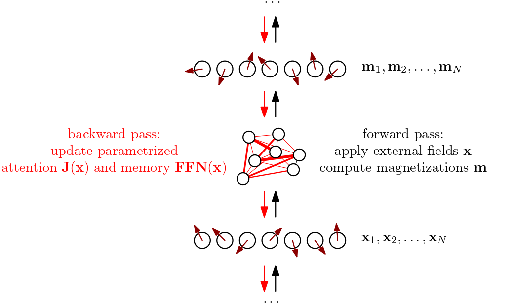
In Spin-Model Transformers (2023), we observed that these systems tend to settle into nonequilibrium steady states (NESSs) as dynamic sweet spots where the “continuous kicking” of the inputs (applied external fields) “sustains” the outputs (magnetizations). This negotiation process tends to happen after just a few iterations. The first iteration already gives a decent guess, which might explain why (1) transformers can get away with stacking modules whose forward passes take just one time step, and (2) why doing a few time steps can improve performance, as done in looping and recursive reasoning approaches. Indeed, repeating the same module can be seen as allowing the underlying nonequilibrium system to settle more snuggly into its steady state for that particular configuration of inputs and parameters. However, as soon as the input drive changes, or the parameters change, the system has to somehow renegotiate a different steady state compatible with what its new configuration dictates the response should be. More on that later (it is more intricate than this; it always is).
Nonequilibrium spin-model transformers
Minimal model
When designing neural networks around mean-field vector-spin models, there is a lot of architectural freedom. First of all, we must decide on what mean-field approximation to use to approximate the time-dependent behavior of our vector-spin system. Projecting the dynamics to different ansatz distributions leads to different mean-field equations, which take into account more or less correlations at different time steps.
Mindful of the importance of locality and scaling in distributed systems, we pick the simplest option: a first-order Plefka[t-1,t] approximation. From Spin-Model Transformers (2023), we all remember
where $\mathbf{m}_{i,t} \in \mathbb{R}^{D}$ denote the magnetizations (outputs) at time $t$, $\mathbf{x}_{i,t} \in \mathbb{R}^{D}$ denote the applied external fields (inputs) at time $t$, $J_{ij}$ are the couplings, $\beta$ is an inverse temperature, and $R=\sqrt{D/2 -1}$ is a natural hyperspherical length scale resulting from the large-$D$ approximation we used to get rid of dealing with Bessel functions. The large-$D$ approximation should be fine since the embedding dimensions in modern neural networks are large.
If we now consider some kind of parametrized drive-dependent couplings
\begin{equation} \mathbf{J} (\mathbf{x}) = \mathrm{softmax}\left( \mathbf{x} \boldsymbol{Q} \boldsymbol{K}^{T} \mathbf{x}^{T} \right), \label{eq:softmax} \end{equation}we turn the fixed-size coupling matrix into a parametrized rule that supports variable system size, drive-dependent routing, and a way to scale system size without learning new explicit parameters. Softmax attention is a convenient choice for a bounded positive row-stochastic coupling rule. Other possible choices include additive or multiplicative combinations with slower base coupling parameters $\mathbf{J}^{0}$ that are drive-independent, leading to a system with persistent interactions in the absence of a drive.
If we also augment the applied external fields with some kind of parametrized drive-dependent local drive or memory,
\begin{equation} \mathbf{x}_{i,t} \to \mathbf{x}_{i,t} + \mathrm{FFN}\left( \mathbf{x}_{i,t} \right), \end{equation}then our forward pass looks like the recurrence relation
\begin{equation} \mathbf{m}_{i,t} = \frac{\beta \left( \mathbf{x}_{i,t} + \mathrm{FFN}\left( \mathbf{x}_{i,t} \right) + \sum_{j} J_{ij} (\mathbf{x}_{t}) \mathbf{m}_{j,t-1} \right)}{1+\sqrt{1+\beta^2 \lVert \mathbf{x}_{i,t} + \mathrm{FFN}\left( \mathbf{x}_{i,t} \right) + \sum_{j} J_{ij} (\mathbf{x}_{t}) \mathbf{m}_{j,t-1} \rVert^2 / R^2 }}, \end{equation}which resembles a parallel transformer block, with the notable difference that the “values” here correspond to the outputs (magnetizations) of the previous time step instead of some linear transformation applied to the inputs at the current time step: current drive routes previous state. Making the applied external fields as well as the couplings drive-dependent leads to a highly-adaptive system where the interaction landscape itself is dynamically shaped by the inputs. Each vector spin effectively experiences a local mean-field that is the sum of a residual stream, a feed-forward-like drive, and attention-like couplings.
But where are the values we know and love from QKV attention? Let us jump ahead and try to figure out what is going on by thinking how we can approach spin-transformer modules. We will be forced to grapple with nonequilibrium thermodynamics (audience groans and starts rolling their eyes). There are two main implementation scenarios: (1) a fixed-point module where we clamp the drive $\mathbf{x}_{t}$ and relax the response along an internal time dimension towards a NESS, and (2) a finite-step recurrent module where changing input drives repeatedly induce quenches or driven transitions. These two limits are about timescale separation and adiabaticity: if the physical drive timescale becomes comparable to the internal relaxation time, then a fixed point is out of reach. When a system is driven rapidly, it fails to relax to an instantaneous NESS and it is forced to keep chasing moving targets in a fast, non-adiabatic regime.
Let us walk through the fixed-point relaxation scenario. Freezing the drive at $\mathbf{x}_{t}$, we interpret the update equations as an inner-loop relaxation
\begin{equation} \mathbf{m}_{i,k} = \frac{\beta \left( \mathbf{x}_{i,t} + \mathrm{FFN}\left( \mathbf{x}_{i,t} \right) + \sum_{j} J_{ij} (\mathbf{x}_{t}) \mathbf{m}_{j,k-1} \right)}{1+\sqrt{1+\beta^2 \lVert \mathbf{x}_{i,t} + \mathrm{FFN}\left( \mathbf{x}_{i,t} \right) + \sum_{j} J_{ij} (\mathbf{x}_{t}) \mathbf{m}_{j,k-1} \rVert^2 / R^2 }}, \end{equation}hopefully settling into an instantaneous near-equilibrium steady-state (NESS) fixed point $\mathbf{m}^{*}_{t}(\mathbf{x}_{t})$ for $k \to \infty$ compatible with the current drive $\mathbf{x}_{t}$. If the fixed point is unique, the influence of the initialization is erased. However, if the landscape is funky, supporting multiple attractor basins or showing signs of hysteresis, then the response $\mathbf{m}^{*}_{t}(\mathbf{x}_{t})$ of the relaxation dynamics does depend on the initialization: the system contains an implicit memory. In this setup, we can interpret values in QKV attention in a transformer block as amortized feed-forward responses, approximating the internal relaxation process by learning a linear mapping, like a one-shot learned estimator of a fixed-point relaxation response. This approach is also reminiscent of deep equilibrium models (DEQs) and looped, recursive reasoning approaches, but, arguably, less ad hoc since here the iterations are done to solve self-consistent mean-field message-passing equations. External time $t$ advances only when the drive changes $\mathbf{x}_{t} \to \mathbf{x}_{t+1}$ (a new sequence arrives) and the nonstationarity messes up everything again, provoking a transition $\mathbf{m}^{*}_{t}(\mathbf{x}_{t}) \to \mathbf{m}^{*}_{t+1}(\mathbf{x}_{t+1})$ between two NESSs.
The second scenario with a finite-step recurrent module is much more challenging. In that case, the driven nonstationary system keeps track of state $\mathbf{m}_{t-1}$ while chasing a moving target with only a finite number of internal relaxation steps for every external time step $t$.
About time and clocks: In this section, we have introduced an external physical time index $t$ as well as an internal relaxation index $k$. Yet at this point we are still only discussing a single module, i.e. a single spin system, getting probed by an environment. A deep network is a stack of untied modules, which, in our framework, are part of a collective of different driven spin systems driving each other sequentially. The layer index does not (have to) correspond to external time nor to internal relaxation time; it is an additional axis labeling the simple feed-forward topology (depth) of the computational graph.
Mean-field proxy for entropy production
Following Aguilera et al. (2020), the housekeeping entropy production for the kinetic Ising model, assuming a nonequilibrium steady state, is given by
\begin{equation} \langle \sigma_{t} \rangle = \sum_{ij} \left(J_{ij} - J_{ji}\right) D_{ij,t} \geq 0, \label{eq:sigma_hk} \end{equation}where $J_{ij}$ corresponds to the couplings and $D_{ij,t}$ denotes the time-delayed correlations. Intuitively, this is like
\begin{equation} \langle \sigma_{t} \rangle = \sum_{ij} \left[\operatorname{directionality}\right]_{ij} \times \left[\operatorname{delayed\ flow}\right]_{ij,t}, \end{equation}or, even more hand-wavy, $\operatorname{dissipation} \sim \operatorname{force} \times \operatorname{flux}$. The asymmetric part of the couplings says whether that propagation channel is directionally biased. The full sum rewards directed, temporally effective, vector-aligned information flow.
Back to reality. If we write down $D_{ij,t}$ for the vector-spin case,
\begin{equation} D_{ij,t} = \int \mathrm{d} \mathbf{s}_{t} \int \mathrm{d} \mathbf{s}_{t-1} \; \left( \mathbf{s}_{i,t} - \mathbf{m}_{i,t} \right) \cdot \left( \mathbf{s}_{j,t-1} - \mathbf{m}_{j,t-1}\right) \; P( \mathbf{s}_{t}, \mathbf{s}_{t-1} ), \end{equation}we can compute a first-order Plefka[t-1,t] mean-field approximation for the time-delayed correlations, similar to the computations we did previously for the magnetizations in Spin-Model Transformers (2023), leading to something like
where $\Sigma_{i,t} = \operatorname{Var} \left[ s_{i,t} \right]$ denotes the single-site covariance / susceptibility. The trace captures which directions on the vector-spin sphere are still available to fluctuate. If a spin is weakly magnetized, it has many soft directions. If it is strongly magnetized, many directions are suppressed because the spin is pinned close to its mean direction.
Substituting the large-$D$ approximation
\begin{align} \Sigma_{i,t} \approx \frac{1}{1+\gamma_{i,t}} - \frac{\mathbf{m}_{i,t} \mathbf{m}_{i,t}^{T}}{R^2 \gamma_{i,t}}, \end{align}we end up with the explicit expression
\begin{align} D_{ij,t} = &\frac{\beta J_{ij}}{1+\gamma_{i,t}} \left(R^2 - \mathbf{m}_{j,t-1}^2 \right) \nonumber\\\\ &- \frac{\beta J_{ij}}{R^2 \gamma_{i,t} \left( 1 + \gamma_{j,t-1} \right)} \mathbf{m}_{i,t}^2 \nonumber\\\\ &+ \frac{\beta J_{ij}}{R^4 \gamma_{i,t} \gamma_{j,t-1}} \left( \mathbf{m}_{i,t} \cdot \mathbf{m}_{j,t-1} \right)^2, \end{align}where
\begin{align} \gamma_{i,t} &= \sqrt{1 + \beta^2 \lVert \boldsymbol{\theta}_{i,t} \rVert^2 / R^2 } \\\\ \boldsymbol{\theta}_{i,t} &= \mathbf{x}_{i,t} + \sum_{j} J_{ij} \mathbf{m}_{j,t-1}. \end{align}The first-order time-delayed correlations $D_{ij,t}$ is a mean-field estimate of how much the fluctuation in one vector spin is transmitted one time step later “into” another spin. Or, put differently, when spin $j$ fluctuates away from its mean at the previous time step $t-1$, how much of that fluctuation shows up as a fluctuation of spin $i$ at the current time step $t$?
Waving hands and checking vibes
Let us try to get a feel for what the entropy production looks like for vector-spin models using some rough back-of-the-envelope estimations. Assume both vectors $\mathbf{m}_{i,t}$ and $\mathbf{m}_{j,t-1}$ have a norm $\mathcal{O}(R)$, then the time-delayed correlations behave approximately like
\begin{align} D_{ij,t} \sim J_{ij} \cos^2 \alpha_{(i,t)(j,t-1)}, \end{align}where $\alpha_{(i,t)(j,t-1)}$ denotes the angle between the magnetization vectors. So the entropy production looks approximately like
\begin{equation} \langle \sigma_{t} \rangle \sim \sum_{ij} \left(J_{ij}^2 - J_{ij} J_{ji}\right) \cos^2 \alpha_{(i,t)(j,t-1)}, \end{equation}which, in general, is minimized for symmetric coupling matrices or orthogonal embeddings and maximized for fully-asymmetric couplings or (anti-)parallel embeddings.
But for the softmax attention matrix Eq. \eqref{eq:softmax}, we have additional constraints $J_{ij} \geq 0$ as well as a Frobenius norm of $\mathcal{O}(\sqrt{N})$ preventing unbounded growth under maximization. Additionally, imposing a causal mask on the couplings to do autoregressive modeling leads to even more constraints since then the upper triangular part of $J_{ij}$ is fixed to zero. So it feels like maximizing entropy production for causal softmax couplings promotes some kind of compromise between sparse attention (intuitively, if the upper-triangular part is zero then it is favorable to push most of the lower-triangular elements close to zero as well) and clustering of embeddings (weighted maximization of cosine similarity).
Entropy production decompositions
We referred to Eq. \eqref{eq:sigma_hk} as housekeeping entropy production and then never mentioned why we called it that way. Let us think again how we can turn vector-spin models with weird drive-dependent couplings $J_{ij}(\mathbf{x}_{t})$ into a transformer-like neural network. Doing so will force us, once again, to grapple with nonequilibrium thermodynamics (audience now visible annoyed and looking for the exit). In the fixed-point interpretation, the housekeeping entropy production
\begin{equation} \langle \sigma_{t} \rangle = \sum_{ij} \left(J_{ij}(\mathbf{x}_{t}) - J_{ji}(\mathbf{x}_{t})\right) D_{ij,t} \end{equation}measures instantaneous local irreversibility of the frozen driven system under the clamped drive $\mathbf{x}_{t}$. Physically, the environment pushes on the module with $\mathbf{x}_{t}$ and the module rapidly relaxes to a NESS characterized by $\mathbf{m}^{*}_{t}(\mathbf{x}_{t})$.
As soon as the drive changes $\mathbf{x}_{t-1} \to \mathbf{x}_{t}$, things get hard. If the drive steps are small, we could end up in an adiabatic regime connecting a sequence of (relaxed) NESSs. But in practice the jump is likely never small and there will be excess contributions from the drive changing. So we end up with a process that is genuinely nonstationary and the steady-state expression no longer gives the complete picture in terms of entropy production.
…
Local-learning rules and sparse credit assignment
…
Imagine we want to turn our entropy production proxy into a loss function. One option would be a stop-gradient / local version
\begin{equation} \langle \sigma_{t} \rangle = \sum_{ij} \left(J_{ij} - J_{ji}\right) \operatorname{sg}\left(D_{ij,t}\right), \end{equation}then $\Delta J_{ij} \propto D_{ij} - D_{ji}$ is a temporally asymmetric Hebbian learning rule.
…
Collectives, loops, and adaptive systems
…
Each module is a driven nonequilibrium response system. It receives boundary conditions from other systems or the environment, relaxes to a response, and emits magnetizations that perturb those boundaries. Memory need not be internal to a module; it may reside in the environment or in the closed-loop configuration of coupled modules.
…
Numerical experiments
…
Model behavior in a noisy environment
Cybernetics, interfaces, environments, sensors, controllers, and effectors.
…
Global coherence from local backpropagation
We test a stack of spin-transformer modules in a toy femtoscale online learning setup and try to see if we can make synchronization or specialization happen between the spin-transformer modules when maximizing per-layer entropy-production losses independently. If we detach module outputs after applying each layer, we end up with systems communicating via their boundary interfaces, but without gradients backpropagating through the whole stack. (Pretty unlikely that the entropy-production losses on their own provide enough signal though.)
…
Growing network topologies
…
Discussion and related work
…
Conclusion
…
Acknowledgements
We acknowledge interesting discussions with GPT 5.5, GPT 5.6, and Claude Opus 4.8. Claude Fable 5 refused to cooperate.
References
A non-exhaustive list of references and inspiration includes:
- A unifying framework for mean-field theories of asymmetric kinetic Ising systems by Miguel Aguilera, S. Amin Moosavi, and Hideaki Shimazaki
- The thermodynamics of prediction by Susanne Still, David A. Sivak, Anthony J. Bell, and Gavin E. Crooks
- Three detailed fluctuation theorems by Massimiliano Esposito and Christian Van den Broeck
- Stochastic thermodynamics of learning by Sebastian Goldt and Udo Seifert
- Self-organized fine-tuned response in a driven spin glass by Jacob Mitchell Gold
If you happen to find this work useful, please consider citing it as:
@article{bal2026,
  title   = {Entropy Production in Nonequilibrium Neural Networks},
  author  = {Bal, Matthias},
  year    = {2026},
  month   = {?},
  url     = {https://mcbal.github.io/post/entropy-production-in-nonequilibrium-neural-networks/}
}
Footnotes
