Entropy Production in Non-Equilibrium Neural Networks

Introduction
✨ Disclaimer: This project is open research and a work in progress
✨ GitHub repository:
mcbal/neqnn
Modern large-scale autoregressive language models are impressive system engineering artifacts. Yet they are frozen, with no apparent notion of dynamics unfolding over time. Surfacing in-context learning at inference time through prompt, harness, and environment engineering mitigates the fact that these models are temporal only in so far as information inside their large but finite context windows matches patterns observed during batched offline training stages. Time, and its dynamic memory affordances, is in a sense amortized or compressed away, incentivizing models to overrely on storing relevant patterns into parametric memory instead of sculpting latent low-dimensional structures supporting stable dynamic computation. This has implications for online continual learning, adaptive model deployment, and real-time closed-loop interaction with live systems.
In this post, we build on Spin-Model Transformers (2023) and take the notion of treating neural networks as non-equilibrium thermodynamic systems seriously. We design a physics-inspired transformer module with adaptable couplings and memory parameters based on the naive mean-field dynamics of a class of vector-spin models. The mean-field spin-model interpretation underpinning the architecture enables us to write down a mean-field proxy for entropy production, a thermodynamic quantity measuring irreversibility by quantifying the asymmetry between forward and backward time steps. Since every operation in our spin-transformer module is differentiable, entropy production can be made into a local loss function measuring irreversible flow.
For example, maximizing entropy production incentivizes the system to lean into the external drive by nudging its parameters to dump entropy as fast as possible given constraints. Internally, we imagine the system reshaping itself into ordered structures to enable more efficient dissipation of the internal tension caused by the incoming data stream. We are not interested in maximal dissipation failure modes, but in useful, controlled dissipation aligned with structure in the environment. Ideally, individual modules locally amplify directional delayed flows in parallel, while module connectivity and environment feedback collectively constrain which flows remain stable and useful for the system as a whole. Ideally, as part of this bitter-lesson-pilled self-organization and synchronization story, prediction and world-model-building are not explicit hand-crafted objectives, but develop internally to better keep local irreversible flows useful.
…
Background and intuitions
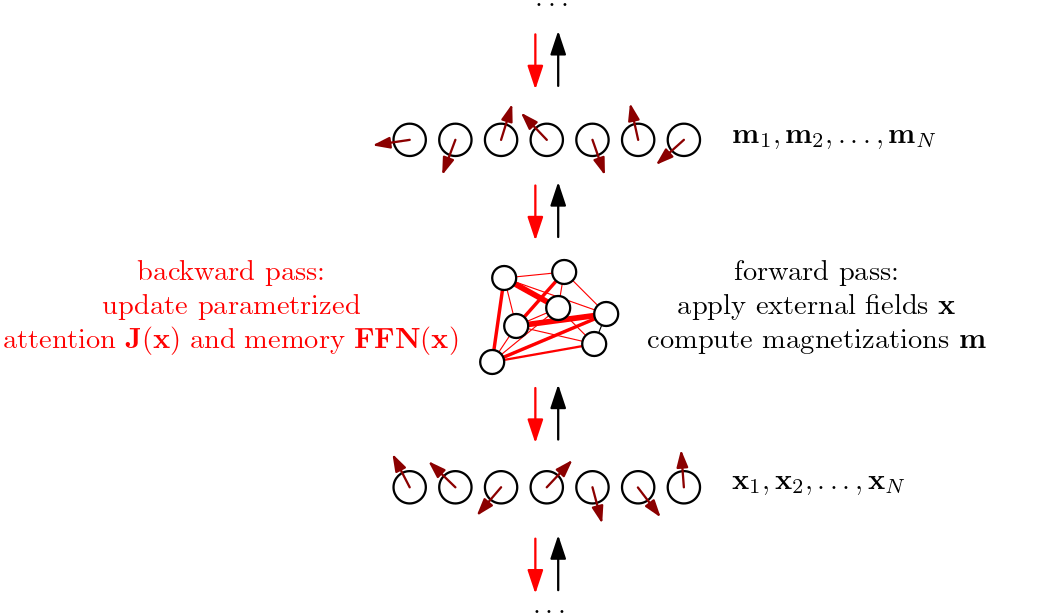
We yet again consider transformer modules as differentiable driven disordered vector-spin systems whose mean-field collective behavior we can control through training, and refer to previous posts going back to Deep Implicit Attention: A Mean-Field Theory Perspective on Attention Mechanisms (2021) for earlier instantiations of this intuition. According to our correspondence, the forward pass of a transformer module implements a spin system’s response to getting probed, where inputs map to time-varying applied external fields, asymmetric, sparse attention matrices can be identified with fully-connected spin-spin interactions, and outputs map to spin expectation values or magnetizations. Practically, the forward pass of a spin-transformer module can be designed to mimic that of a vanilla transformer module.
In contrast to physics-oriented literature, we do not specify explicit probability distributions for the external fields and couplings of the disordered many-body system, nor are we interested in Nobel-prize-winning ways to average out the disorder. We instead focus on the very specific quenched disorder realizations induced by a dataset or environment of interest (encoded as sequences of vector embeddings), whose examples we use to drive the system. In this framing, training a transformer module corresponds to sculpting the underlying system’s collective response by tuning the parametrized distributions of its external fields and couplings.
In Spin-Model Transformers (2023), we observed that these systems tend to settle into non-equilibrium steady states as dynamic sweet spots where the “continuous kicking” of the inputs (applied external fields) “sustains” the outputs (magnetizations). This negotiation process tends to happen after just a few iterations. The first iteration already gives a decent guess, which might explain why (1) transformers can get away with just stacking modules whose forward passes take just one time step, and (2) why doing a few time steps can improve performance, as done in looping and recursive reasoning approaches. Indeed, repeating the same module can be seen as allowing the underlying non-equilibrium system to settle more snuggly into its steady state for that particular configuration of inputs and parameters. However, as soon as the input sequence changes, or the parameters change, the system has to renegotiate a different steady state compatible with what its new configuration dictates the response should be.
…
Non-equilibrium neural networks
Example model
When designing neural networks around mean-field vector-spin models, there is a lot of architectural freedom. First of all, we must decide on what mean-field approximation to use to approximate the time-dependent behavior of our vector-spin system. Projecting the dynamics to different ansatz distributions leads to different mean-field equations, which take into account more or less correlations at different time steps.
Mindful of the importance of locality and scaling, we pick the simplest option: a first-order Plefka[t-1,t] approximation. From Spin-Model Transformers (2023), we all remember
where $\mathbf{m}_{i,t} \in \mathbb{R}^{D}$ denote the magnetizations (outputs) at time $t$, $\mathbf{x}_{i,t} \in \mathbb{R}^{D}$ denote the applied external fields (inputs) at time $t$, $J_{ij}$ are the couplings, $\beta$ is an inverse temperature, and $R=\sqrt{D/2 -1}$ is a natural hyperspherical length scale resulting from the large-$D$ approximation we used to get rid of dealing with Bessel functions. The large-$D$ approximation should be fine since the embedding dimensions in modern neural networks are large.
If we now consider some kind of parametrized input-dependent couplings
\begin{equation} \mathbf{J} (\mathbf{x}) = \mathrm{softmax}\left( \mathbf{x} \boldsymbol{Q} \boldsymbol{K}^{T} \mathbf{x}^{T} \right), \label{eq:softmax} \end{equation}and augment the applied external fields with some kind of parametrized input-dependent local drive or memory,
\begin{equation} \mathbf{x}_{i,t} \to \mathbf{x}_{i,t} + \mathrm{FFN}\left( \mathbf{x}_{i,t} \right), \end{equation}then our forward pass looks like
\begin{equation} \mathbf{m}_{i,t} = \frac{\beta \left( \mathbf{x}_{i,t} + \mathrm{FFN}\left( \mathbf{x}_{i,t} \right) + \sum_{j} J_{ij} (\mathbf{x}_{t}) \mathbf{m}_{j,t-1} \right)}{1+\sqrt{1+\beta^2 \lVert \mathbf{x}_{i,t} + \mathrm{FFN}\left( \mathbf{x}_{i,t} \right) + \sum_{j} J_{ij} (\mathbf{x}_{t}) \mathbf{m}_{j,t-1} \rVert^2 / R^2 }}, \end{equation}which resembles a parallel transformer block, with the notable difference that the “values” here correspond to the outputs (magnetizations) of the previous time step instead of some linear transformation applied to the inputs at the current time step. Making the applied external fields as well as the couplings input-dependent leads to a highly-adaptive system where the interaction landscape itself is dynamically shaped by the inputs. Each vector spin effectively experiences a local mean-field that is the sum of a residual stream, a feed-forward-like drive, and attention-like couplings.
We can choose to have our module keep track of the previous state so that one forward pass corresponds to taking a single time step. If we care more about the steady state, we can also immediately compute the fixed point of the time evolution using a differentiable fixed-point solver. In that case, one forward pass corresponds to jumping to the time-evolution fixed point. The latter approach is reminiscent of deep equilibrium models and recent looped, recursive reasoning approaches, but arguably less ad hoc here since we loop to solve self-consistent mean-field message-passing-likeequations.
Mean-field proxy for entropy production
Following Aguilera et al. (2020), the entropy production for the kinetic Ising model, assuming a non-equilibrium steady state, is given by
\begin{equation} \sigma_{t} = \sum_{ij} \left(J_{ij} - J_{ji}\right) D_{ij,t} \geq 0, \end{equation}where $J_{ij}$ corresponds to the couplings and $D_{ij,t}$ denotes the time-delayed correlations. Intuitively, this is like
\begin{equation} \sigma_{t} = \sum_{ij} \left[\operatorname{directionality}\right]_{ij} \times \left[\operatorname{delayed\ flow}\right]_{ij,t}, \end{equation}or, even more hand-wavy, $\operatorname{dissipation} \sim \operatorname{force} \times \operatorname{flux}$. The asymmetric part of the couplings says whether that propagation channel is directionally biased. The full sum rewards directed, temporally effective, vector-aligned information flow.
Back to reality. If we write down $D_{ij,t}$ for the vector-spin case,
\begin{equation} D_{ij,t} = \int \mathrm{d} \mathbf{s}_{t} \int \mathrm{d} \mathbf{s}_{t-1} \; \left( \mathbf{s}_{i,t} - \mathbf{m}_{i,t} \right) \cdot \left( \mathbf{s}_{j,t-1} - \mathbf{m}_{j,t-1}\right) \; P( \mathbf{s}_{t}, \mathbf{s}_{t-1} ), \end{equation}we can compute a first-order Plefka[t-1,t] mean-field approximation for the time-delayed correlations, similar to the computations we did previously for the magnetizations in Spin-Model Transformers (2023), leading to something like
where $\Sigma_{i,t} = \operatorname{Var} \left[ s_{i,t} \right]$ denotes the single-site covariance. The trace captures which directions on the vector-spin sphere are still free to fluctuate. If a spin is weakly magnetized, it has many soft directions. If it is strongly magnetized, many directions are suppressed because the spin is pinned close to its mean direction.
Substituting the large-$D$ approximation
\begin{align} \Sigma_{i,t} \approx \frac{1}{1+\gamma_{i,t}} - \frac{\mathbf{m}_{i,t} \mathbf{m}_{i,t}^{T}}{R^2 \gamma_{i,t}}, \end{align}we end up with the explicit expression
\begin{align} D_{ij,t} = &\frac{\beta J_{ij}}{1+\gamma_{i,t}} \left(R^2 - \mathbf{m}_{j,t-1}^2 \right) \nonumber\\\\ &- \frac{\beta J_{ij}}{R^2 \gamma_{i,t} \left( 1 + \gamma_{j,t-1} \right)} \mathbf{m}_{i,t}^2 \nonumber\\\\ &+ \frac{\beta J_{ij}}{R^4 \gamma_{i,t} \gamma_{j,t-1}} \left( \mathbf{m}_{i,t} \cdot \mathbf{m}_{j,t-1} \right)^2, \end{align}where
\begin{align} \gamma_{i,t} &= \sqrt{1 + \beta^2 \lVert \boldsymbol{\theta}_{i,t} \rVert^2 / R^2 } \\\\ \boldsymbol{\theta}_{i,t} &= \mathbf{x}_{i,t} + \sum_{j} J_{ij} \mathbf{m}_{j,t-1}. \end{align}The first-order time-delayed correlations $D_{ij,t}$ is a mean-field estimate of how much the fluctuation in one vector spin is transmitted one time step later “into” another spin. Or, put differently, when spin $j$ fluctuates away from its mean at the previous time step $t-1$, how much of that fluctuation shows up as a fluctuation of spin $i$ at the current time step $t$?
Vibe check
Let us try to get a feel for what the entropy production looks like for vector-spin models using some rough back-of-the-envelope estimations. Assume both vectors $\mathbf{m}_{i,t}$ and $\mathbf{m}_{j,t-1}$ have a norm $\mathcal{O}(R)$, then the time-delayed correlations behave approximately like
\begin{align} D_{ij,t} \sim J_{ij} \cos^2 \alpha_{(i,t)(j,t-1)}, \end{align}where $\alpha_{(i,t)(j,t-1)}$ denotes the angle between the magnetization vectors. So the entropy production looks approximately like
\begin{equation} \sigma_{t} \sim \sum_{ij} \left(J_{ij}^2 - J_{ij} J_{ji}\right) \cos^2 \alpha_{(i,t)(j,t-1)}, \end{equation}which, in general, is minimized for symmetric coupling matrices or orthogonal embeddings and maximized for fully-asymmetric couplings or (anti-)parallel embeddings.
But for the softmax attention matrix Eq. \eqref{eq:softmax}, we have additional constraints $J_{ij} \geq 0$ as well as a Frobenius norm of $\mathcal{O}(\sqrt{N})$ preventing unbounded growth under maximization. Additionally, imposing a causal mask on the couplings to do autoregressive modeling leads to even more constraints since then the upper triangular part of $J_{ij}$ is fixed to zero. So it feels like maximizing entropy production for causal softmax couplings promotes some kind of compromise between sparse attention (intuitively, if the upper-triangular part is zero then it is favorable to push the lower-triangular elements close to zero as well) and clustering of embeddings (weighted maximization of cosine similarity).
✨ The mean-field entropy production proxy captures how much asymmetric attention transports aligned state fluctuations forward in time.
…
Local-learning rules and sparse credit assignment
…
Imagine we want to turn our entropy production proxy into a loss function. One option would be a stop-gradient / local version
\begin{equation} \sigma_{t} = \sum_{ij} \left(J_{ij} - J_{ji}\right) \operatorname{sg}\left(D_{ij,t}\right), \end{equation}then $\Delta J_{ij} \propto D_{ij} - D_{ji}$ is a temporally asymmetric Hebbian learning rule.
…
Numerical experiments
…
Model behavior in a noisy environment
Cybernetics, interfaces, environments, sensors, controllers, and effectors.
…
Global coherence from local backpropagation
We test a stack of spin-transformer modules in a toy femtoscale online learning setup and try to see if we can make synchronization happen between the spin-transformer modules when maximizing per-layer entropy-production losses independently. If we detach module outputs after applying each layer, we end up with systems communicating via their input/output interfaces but without gradients backpropagating through the whole stack. (Pretty unlikely that the entropy-production losses on their own provide enough signal though.)
…
Growing network topologies
…
Discussion and related work
…
References
A non-exhaustive list of references and inspiration includes:
- A unifying framework for mean-field theories of asymmetric kinetic Ising systems by Miguel Aguilera, S. Amin Moosavi, and Hideaki Shimazaki
- Self-organized fine-tuned response in a driven spin glass by Jacob Mitchell Gold
- Bootstrapping Life-Inspired Machine Intelligence: The Biological Route from Chemistry to Cognition and Creativity by Giovanni Pezzulo and Michael Levin
If you happen to find this work useful, please consider citing it as:
@article{bal2026,
  title   = {Entropy Production in Non-Equilibrium Neural Networks},
  author  = {Bal, Matthias},
  year    = {2026},
  month   = {?},
  url     = {https://mcbal.github.io/post/entropy-production-in-non-equilibrium-neural-networks/}
}
Footnotes
