
Introduction
✨ Code:
mcbal/large-d-closure
In previous posts, we built transformer-like modules around naive mean-field descriptions of driven stochastic vector spins wobbling about on hyperspheres. The modules behaved well as part of a toy language model, but their mean-field observables showed persistent errors compared to exact sampling of the stochastic system, especially in delayed correlations and at lower temperatures, even as the vector dimension $D$ grew. Rather than turning to second-order (TAP) mean-field approximations, which for vector spins lead to implicit fixed-point equations at every update, we ask whether the geometry of high-dimensional spheres can on its own provide a more faithful approximation for a fixed realization of couplings and drives.
The motivation for taking the large-$D$ limit comes from the structure of attention modules, which act on a context window of $N$ tokens with a large head or model dimension $D$. Softmax couplings are computed from the inputs and held fixed within a forward pass. Crucially, attention can be sharp or diffuse for different tokens in the same context, regardless of the context length. So we want an approximation that works whether a site effectively interacts with one input or with many. We let $D\to\infty$ at fixed $N$ and fixed couplings, without requiring $D \gg N$. What matters is a site’s effective number of interaction partners rather than the context length, which, in practice, can far exceed $D$.
Physically, each vector spin responds to a field made up of a local drive plus its neighbors weighted by the couplings. Mean field averages the neighbors before applying the response, which ignores fluctuations on the hypersphere. Yet the strength of a spin’s alignment depends on the length of its field, and thus on the missing contributions of the fluctuations. We show that the squared field length concentrates for large $D$, but around a value that includes the fluctuations rather than around its bare mean-field value. Taking this into account yields a closure: a set of explicit recurrence relations for means and covariance traces at equal and consecutive times. We find numerically that the closure’s errors fall off roughly as $1/D$, while those of naive mean field level off. For a single update, the correction costs one extra pass with squared attention weights.
Background
Stochastic model dynamics
Consider $N$ spins $\mathbf s_i\in\mathbb R^D$ of length $R$, with $R^2=D/2-1$1 and $D>2$. Fixed scalar couplings $J_{ij}$ mix the spins, and fixed fields $\mathbf x_i$ drive them. The couplings may be asymmetric, and we do not assume anything about their statistics. All sites are updated synchronously and independently, given the current state:
\begin{equation} P(\mathbf S'\mid\mathbf S)=\prod_i\frac{e^{\beta\,\mathbf s_i'\cdot\mathbf h_i}}{\mathcal Z(\mathbf h_i)}, \qquad \mathbf h_i=\mathbf x_i+\sum_jJ_{ij}\mathbf s_j, \end{equation}where $\beta > 0$ denotes the inverse temperature. The local conditional distribution at each site is a von Mises–Fisher (vMF) distribution, with mean direction $\hat{\mathbf h}_i$ and concentration parameter $\kappa_i=\beta R\lVert\mathbf h_i\rVert$. We will send $D\to\infty$ at fixed $N$, $J_{ij}$, and $\beta$, holding the ratio $\beta\lVert\mathbf x_i\rVert/R$ fixed. Drives of length $O(\sqrt D)$ can then compete with the interaction field, and conditional concentrations $\kappa_i$ are $O(D)$. We start from spins drawn independently from prescribed vMF distributions.
On fluctuating spins. Across stochastic trajectories, the spins $\mathbf s$, and therefore the fields $\mathbf h$, fluctuate. The synchronous update happens in two steps: the current spins determine the fields, which then condition the vMF distributions the next spins are sampled from.
High-dimensional vMF geometry
At $\kappa\propto D$, typical vMF samples occupy a thin ring at a fixed latitude around the field direction, with the mean at its center, see Figure 1(a) and Appendix A. Why a ring? The field favors alignment, but the hypersphere in high dimensions offers vastly more room near the equator than near the pole. At $\kappa\propto D$, these effects balance at a fixed latitude. Increasing $D$ then sharpens the ring without shrinking it, see Figure 1(b).
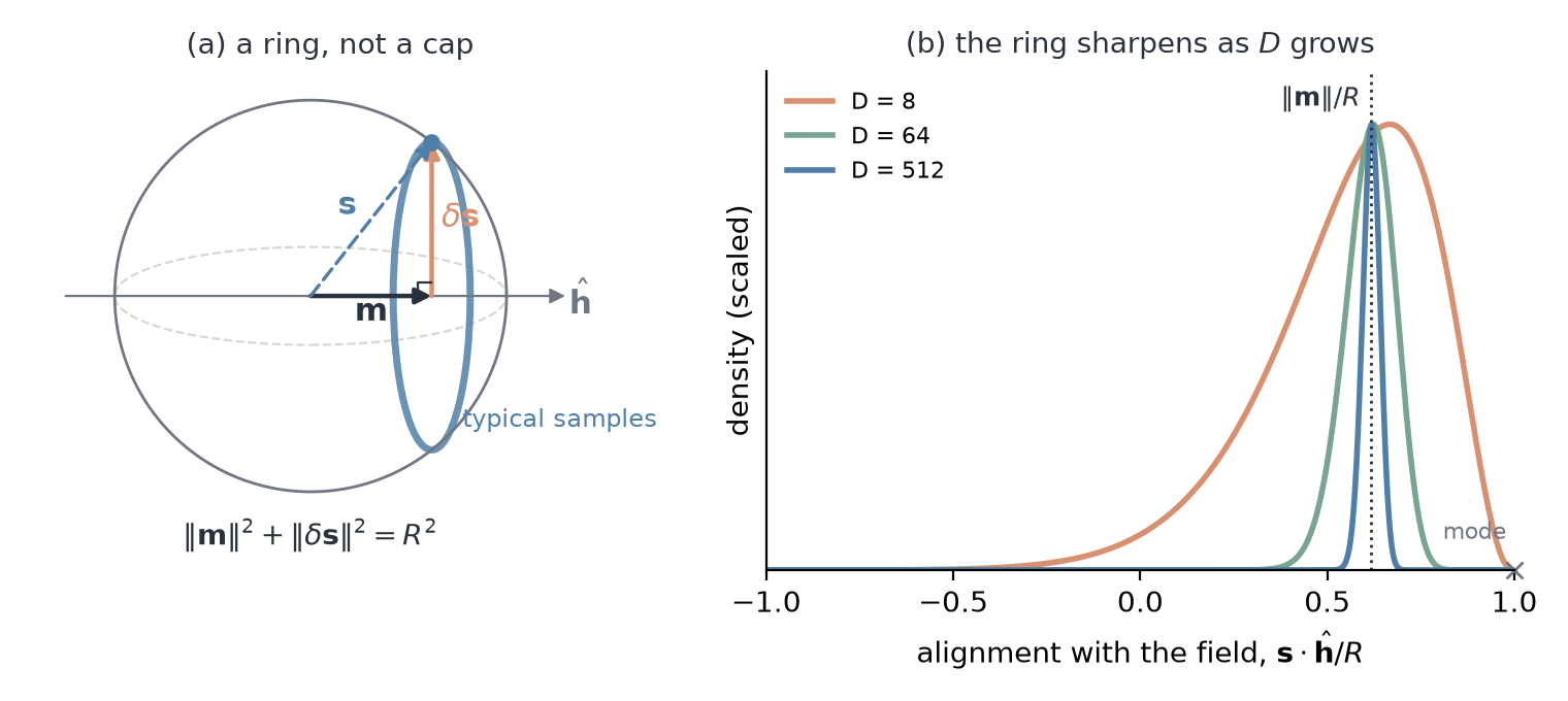
A fluctuation $\delta\mathbf s=\mathbf s-\mathbf m$ about the vMF mean $\mathbf m$ has squared length $O(D)$, spread out mainly over $D-1$ transverse directions, with $O(1)$ variance along any unit direction (see Appendix B). It is nearly perpendicular to the mean, so $\lVert\mathbf m\rVert^2+\lVert\delta\mathbf s\rVert^2\simeq R^2$. Even though the low-dimensional cartoon suggests otherwise, independent fluctuations, of one spin or of different spins, are nearly orthogonal, so their squared lengths add.
Single-spin response
For a given field $\mathbf h$, the exact conditional vMF mean of the next spin is $\boldsymbol\mu_D(\mathbf h)=R A_D(\kappa)\hat{\mathbf h}$, where $A_D(\kappa)=I_{D/2}(\kappa)/I_{D/2-1}(\kappa)$ is a ratio of modified Bessel functions. To get rid of Bessel functions, we consider the leading large-$D$ form
\begin{equation} \boldsymbol\mu_D(\mathbf h) \simeq g(\lVert\mathbf h\rVert^2)\,\mathbf h, \label{eq:response} \end{equation}where the nonlinear gain function is given by
\begin{equation} g(r^2)=\frac{\beta}{1+\gamma(r^2)}, \qquad \gamma(r^2)=\sqrt{1+\beta^2r^2/R^2}. \end{equation}This coincides with the response map $\varphi_\beta$ used in Spin-Model Transformers.
Two properties of the (large-$D$) single-spin response will be useful later on: (1) the gain function depends only on the field norm, and (2) the sphere geometry fixes the conditional variance,
\begin{equation} \mathbb E\!\left[\lVert\mathbf s'-\boldsymbol\mu_D(\mathbf h)\rVert^2\mid\mathbf h\right] =R^2-\lVert\boldsymbol\mu_D(\mathbf h)\rVert^2 \simeq\frac{2R^2}{1+\gamma}. \end{equation}On wobbling spins. Appendix B provides the full covariance and also shows that the exact gain $RA_D(\kappa)/\lVert\mathbf h\rVert$ equals $\beta\tau$, where $\tau$ is the variance along any transverse direction. Our $g$ is its leading-order form, accurate to a relative $O(1/D)$. Intuitively, the gain is the spin’s transverse susceptibility: nudging the field sideways drags the mean along with it, and by fluctuation–response that susceptibility equals $\beta$ times the sideways variance. Note that $g$ is a response per unit field: it decreases with field strength, while the alignment $g\lVert\mathbf h\rVert/R$ still increases. The sphere ties alignment and wobble together: a more strongly aligned, more “pinned” spin wobbles less, in every direction.
The large-D closure
Let us first split the fluctuating spin into $\mathbf s_i=\mathbf m_i+\delta\mathbf s_i$, with $\mathbf m_i=\mathbb E\left[\mathbf s_i\right]$, where expectations are over the spin dynamics at fixed $J$ and $\mathbf x$. We collect the equal-time covariance traces in an $N\times N$ matrix $C$. Each entry is the trace over vector components of the $D\times D$ cross-covariance matrix:
\begin{equation} C_{ij}=\operatorname{tr}\mathbb E\!\left[\delta\mathbf s_i\delta\mathbf s_j^\top\right] =\mathbb E\!\left[\delta\mathbf s_i\cdot\delta\mathbf s_j\right]. \end{equation}The field splits similarly into its mean and fluctuation,
\begin{equation} \mathbf h_i=\bar{\mathbf h}_i+\boldsymbol\eta_i, \qquad \bar{\mathbf h}_i=\mathbf x_i+\sum_jJ_{ij}\mathbf m_j, \qquad \boldsymbol\eta_i=\sum_jJ_{ij}\delta\mathbf s_j. \end{equation}Naive mean field drops $\boldsymbol\eta_i$ and replaces the average of the response
\begin{equation} \mathbf m_i'=\mathbb E[\mathbf s_i']=\mathbb E_{\mathbf h_i} \big[\boldsymbol\mu_D(\mathbf h_i)\big] \end{equation}with the response to the average field
\begin{equation} \mathbf m_i'=\boldsymbol\mu_D(\bar{\mathbf h}_i). \end{equation}But as we have learned from high-dimensional vMF geometry, these fluctuations can take up as much squared length as the mean field, or more.
Typical field length
So what is the length of the typical field? Let us split off the noise,
\begin{equation} \lVert\mathbf h_i\rVert^2=\lVert\bar{\mathbf h}_i\rVert^2+2\,\bar{\mathbf h}_i\cdot\boldsymbol\eta_i+\lVert\boldsymbol\eta_i\rVert^2. \end{equation}The cross term averages to zero, since the noise has zero mean. Its fluctuations are only $O(\sqrt D)$, since the noise has $O(1)$ variance along $\bar{\mathbf h}_i$. The squared noise length, by contrast, has a mean of order $D$. The squared lengths of the mean-field and noise vectors add just like in Figure 1:
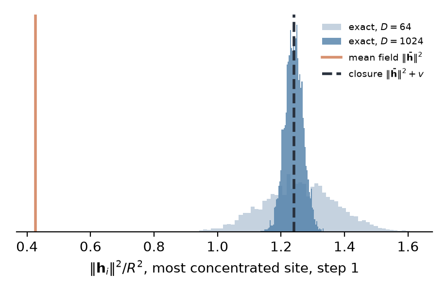
\begin{equation} \mathbb E\lVert\mathbf h_i\rVert^2 =\lVert\bar{\mathbf h}_i\rVert^2+v_i\equiv r_i^2, \qquad v_i=\mathbb E\lVert\boldsymbol\eta_i\rVert^2=(JCJ^\top)_{ii}. \end{equation}Even though both $\lVert\bar{\mathbf h}_i\rVert^2$ and $v_i$ can be $O(D)$, the fluctuations around their sum are only $O(\sqrt D)$. Can we understand this intuitively? Expanding $\mathbf h_i$, the normalized squared field length is a fixed combination of normalized overlaps $\mathbf s_j\cdot\mathbf s_l/R^2$ and $\mathbf x_i\cdot\mathbf s_j/R^2$. For independent spins, these overlaps fluctuate by only $O(D^{-1/2})$, since every spin has $O(1)$ variance along any fixed direction. After an update, shared inputs correlate the spins, but given the current spins, the fresh draws are still independent across sites, which carries the same scaling over to the next update. At any fixed number of updates, we therefore have2
\begin{equation} \operatorname{std}\!\left(\frac{\lVert\mathbf h_i\rVert^2}{R^2}\right)=O(D^{-1/2}). \end{equation}Figure 2 checks this numerically with samples of the squared field norm for a site in a simulated system with $N=256$ vector spins. The squared-norm distribution clearly narrows around $r_i^2$, and not around the mean-field value $\lVert\bar{\mathbf h}_i\rVert^2$.
A deterministic gain…
In the response of Eq. \eqref{eq:response}, the field’s direction fluctuates, but its squared length concentrates around $r_i^2$. The gain $g$, which only depends on the norm, therefore becomes effectively deterministic at large $D$. We can approximate it by
\begin{equation} a_i=g(r_i^2)=\frac{\beta}{1+\gamma_i}, \qquad \gamma_i=\sqrt{1+\beta^2r_i^2/R^2}. \end{equation}This makes the mean response a simple deterministic rescaling of the field.
… and a lot of noise
The next spin is then approximately3
\begin{equation} \mathbf s_i'\simeq \underbrace{a_i\bar{\mathbf h}_i}_{\text{next mean}} +\underbrace{a_i\boldsymbol\eta_i}_{\text{propagated noise}} +\underbrace{\boldsymbol\epsilon_i}_{\text{fresh noise}}. \label{eq:linear} \end{equation}Here $\boldsymbol\eta_i=\sum_jJ_{ij}\delta\mathbf s_j$ is the noise already present in the inputs. The fresh noise $\boldsymbol\epsilon_i=\mathbf s_i'-\boldsymbol\mu_D(\mathbf h_i)$ comes from drawing a spin around its conditional mean. Both noise terms average to zero, giving our first closure relation $\mathbf m_i'\simeq a_i\bar{\mathbf h}_i$.
What remains is the next fluctuation, $\delta\mathbf s_i'\simeq a_i\boldsymbol\eta_i+\boldsymbol\epsilon_i$. Pairing two of these gives the next covariance traces, and pairing one with a current fluctuation gives the one-step delayed covariance $\mathcal D_{ij}=\mathbb E[\delta\mathbf s_i'\cdot\delta\mathbf s_j]$:
\begin{equation} \begin{aligned} C_{ij}'&\simeq a_ia_j\,\mathbb E[\boldsymbol\eta_i\cdot\boldsymbol\eta_j] +a_i\,\mathbb E[\boldsymbol\eta_i\cdot\boldsymbol\epsilon_j] +a_j\,\mathbb E[\boldsymbol\epsilon_i\cdot\boldsymbol\eta_j] +\mathbb E[\boldsymbol\epsilon_i\cdot\boldsymbol\epsilon_j],\\ \mathcal D_{ij}&\simeq a_i\,\mathbb E[\boldsymbol\eta_i\cdot\delta\mathbf s_j] +\mathbb E[\boldsymbol\epsilon_i\cdot\delta\mathbf s_j]. \end{aligned} \end{equation}The two kinds of noise contribute differently:
Propagated noise. Mixing the old fluctuations through $J$ gives $\mathbb E[\boldsymbol\eta_i\cdot\boldsymbol\eta_j]=\sum_{lm}J_{il}J_{jm}C_{lm}=(JCJ^\top)_{ij}$ and $\mathbb E[\boldsymbol\eta_i\cdot\delta\mathbf s_j]=(JC)_{ij}$. The gains then rescale these by $a_ia_j$ and $a_i$.
Fresh noise. Given the old spins, $\boldsymbol\epsilon_i$ has zero mean, while $\boldsymbol\eta_j$ and $\delta\mathbf s_j$ are fixed. Every term pairing fresh noise with old fluctuations therefore vanishes, and only propagated noise correlates with the current state. Each site also draws independently, so $\mathbb E[\boldsymbol\epsilon_i\cdot\boldsymbol\epsilon_j]=0$ for $i\neq j$. Fresh noise only adds to the diagonal. How much? Well, every new spin has squared length $R^2$, which means we have $\mathbb E\lVert\boldsymbol\epsilon_i\rVert^2=R^2-\mathbb E\lVert\boldsymbol\mu_D(\mathbf h_i)\rVert^2$ exactly. The conditional mean has typical squared length $a_i^2r_i^2$, so we approximate the remaining variance by
\begin{equation} b_i\equiv R^2-a_i^2r_i^2=\frac{2R^2}{1+\gamma_i}. \end{equation}Adding the propagated input noise gives the total variance at a site:
\begin{equation} C_{ii}'\simeq\underbrace{a_i^2v_i}_{\text{propagated noise variance}}+\underbrace{b_i}_{\text{fresh noise variance}}. \end{equation}Closure equations
Combining these pieces, with $A=\mathrm{diag}(a)$, gives the full closure equations:
\begin{equation} \boxed{ \begin{aligned} \mathbf m_i'&=a_i\bar{\mathbf h}_i,\\ C'&=AJCJ^\top A+\mathrm{diag}(b),\\ \mathcal D&=AJC. \end{aligned}} \label{eq:closure} \end{equation}So why do the moments close? At large $D$, concentration makes the response gains effectively deterministic. With these gains fixed, spins propagate linearly, and fresh draws supply conditionally centered noise that is uncorrelated across sites. The mean and covariance recursions then follow from linear moment propagation, and the gains remain determined self-consistently by those moments. The main approximation is therefore replacing fluctuating gains by their concentrated values, see Appendix C.
By construction of $b_i$, the equations preserve the spin’s squared length:
\begin{equation} \lVert\mathbf m_i'\rVert^2+C_{ii}' =a_i^2\bigl(\lVert\bar{\mathbf h}_i\rVert^2+v_i\bigr)+b_i=R^2. \end{equation}In each trajectory, the conditional mean $\boldsymbol\mu_D(\mathbf h_i)\simeq a_i\mathbf h_i$ has squared length close to $a_i^2r_i^2$, but its direction varies with $\boldsymbol\eta_i$. Averaging over trajectories cancels these sideways parts and leaves $\mathbf m_i'=a_i\bar{\mathbf h}_i$, of squared length $a_i^2\lVert\bar{\mathbf h}_i\rVert^2$. The difference, $a_i^2v_i$, is the spread of the conditional means across trajectories, which is the propagated noise variance. Fresh noise, the spread around each conditional mean, fills up the rest.
What mean field misses
Now that we have an idea of the effect of the noise, we can pinpoint the failure modes of naive mean field and how the closure addresses them.
Norm inflation. Including $v_i$ lowers the gain, shortening the next mean for a given mean field $\bar{\mathbf h}_i$. By dropping $v_i$, mean field inflates its norm. At strong fields $\beta r_i/R\gg1$, we have that $a_i\simeq R/r_i$, so $\mathbf m_i'\simeq R\,\bar{\mathbf h}_i/r_i$: the closure normalizes the mean field by the full field length $r_i$. Naive mean field instead divides by $\lVert\bar{\mathbf h}_i\rVert$ in its own strong-field limit, $\beta\lVert\bar{\mathbf h}_i\rVert/R\gg1$. From a product start, only individual input variances contribute, so
\begin{equation} v_i=\sum_jJ_{ij}^2\left(R^2-\lVert\mathbf m_{0,j}\rVert^2\right) \leq\frac{R^2}{N_{\mathrm{eff},i}}, \qquad N_{\mathrm{eff},i}=\frac{1}{\sum_jJ_{ij}^2}, \label{eq:first} \end{equation}and norm inflation is bounded by how concentrated the couplings are. For couplings with nonnegative rows summing to one (like softmax attention), the participation ratio counts effective inputs: $N_{\mathrm{eff}}$ ranges from 1 for a single input to $N$ for uniform weights, and equals the number of inputs only when they are weighted equally. Diffuse attention suppresses independent input noise, while sharp attention retains it, so norm inflation is strongest for sharp attention. Since $v_i/R^2$ does not depend on $D$, increasing $D$ alone does not make mean field accurate. For transformer-like applications, we want to maintain accuracy across both regimes.
Shared inputs. After an update, sites talking to the same inputs acquire equal-time covariance. This shared noise feeds back into $v_i$ and contributes to the delayed correlations:
\begin{equation} \mathcal D_{ij}=\underbrace{a_iJ_{ij}C_{jj}}_{\text{direct}} +\underbrace{a_i\sum_{l\neq j}J_{il}C_{lj}}_{\text{shared}}. \end{equation}The shared term can matter even when $J_{ij}$ is small. With nonnegative $J$ and a product start, the closure generates nonnegative entries of $C$, so the two contributions reinforce each other.
Numerical checks
We now compare exact vMF sampling with three recursive approximations. Each propagates its own means through the mean field $\bar{\mathbf h}_i=\mathbf x_i+\sum_jJ_{ij}\mathbf m_j$, with
\begin{equation} a_i=g\bigl(\lVert\bar{\mathbf h}_i\rVert^2+v_i\bigr), \qquad \mathbf m_i'=a_i\bar{\mathbf h}_i, \qquad b_i=\frac{2R^2}{1+\gamma_i}, \end{equation}where $\gamma_i$ is evaluated at the same field length as $a_i$. All three use the leading-order gain $g$ of Eq. \eqref{eq:response} rather than the exact vMF response, so they differ only in the input noise $v_i$ the gain sees and the covariance they carry:
| $v_i$ in the gain | covariance carried | delayed covariance $\mathcal D_{ij}$ | |
|---|---|---|---|
| naive mean field | $0$ | none | linear response, Eq. \eqref{eq:mfdelayed} |
| diagonal closure | $\sum_jJ_{ij}^2C_{jj}$ | diagonal, $C_{ii}'=a_i^2v_i+b_i$ | $a_iJ_{ij}C_{jj}$ |
| full closure | $(JCJ^\top)_{ii}$ | all pairs, Eq. \eqref{eq:closure} | $(AJC)_{ij}$ |
For the delayed correlations of naive mean field, we use the previous post’s linear-response approximation, built from the single-spin covariances $\Sigma(\mathbf h)$ of Appendix B:
\begin{equation} \mathcal D_{ij}=\beta J_{ij}\operatorname{tr}\bigl[\Sigma(\bar{\mathbf h}_i)\,\Sigma_j\bigr], \label{eq:mfdelayed} \end{equation}where $\Sigma_j$ is the covariance of the current spin $j$, evaluated at the mean field that produced it. The diagonal closure (diagonal $C$ in the figures) keeps norm inflation from independent input noise, but drops shared noise. A product start has diagonal $C$, so the two closures give the same means and delayed correlations at the first update. They separate once shared inputs correlate the spins.
Initialization and parameters. Spins start independently in vMF initializer fields. Drives have random directions and strength $\beta\lVert\mathbf x_i\rVert/R=u$. Couplings are a row-wise $\mathrm{softmax}(\alpha G)$ of a fixed Gaussian matrix: increasing $\alpha$ focuses the weights on fewer inputs. Unless stated otherwise, $\beta=2$ and $u=1$. We write $K$ for the number of updates.
Relative errors. Errors are relative Frobenius errors corrected for Monte Carlo noise.4 Mean errors compare overlaps $\mathbf m_i\cdot\mathbf m_j/R^2$ and $\mathbf x_i\cdot\mathbf m_j/R^2$, except where vector errors are stated, including Figure 4(a). Delayed-correlation errors compare $\mathcal D_{ij}/R^2$.
Convergence in D
We first fix $N=256$ and $\alpha=3$, giving $N_{\mathrm{eff}}\approx7.5$ on average, and increase $D$ from 16 to 1024, see Figure 3.
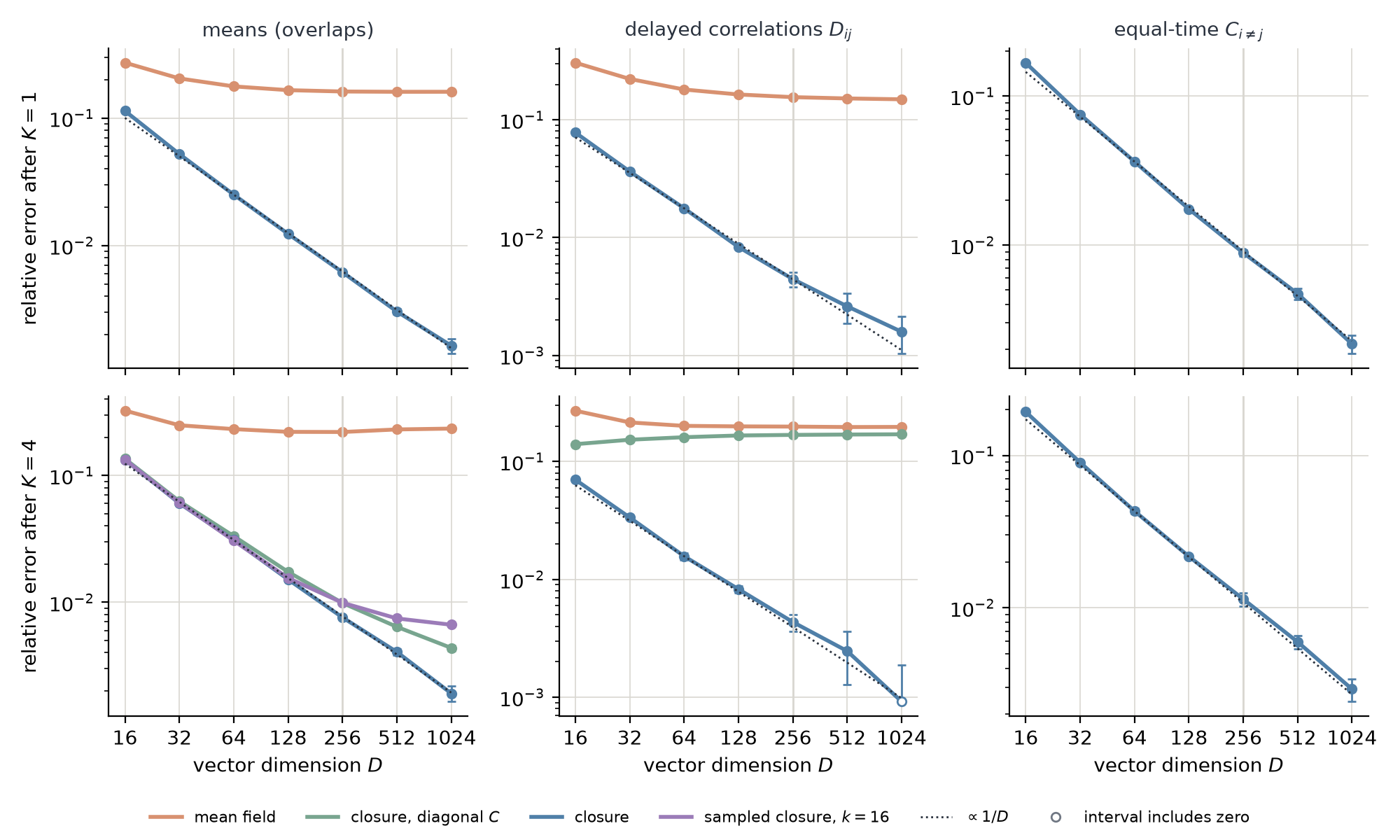
The closure’s resolved errors fall roughly as $1/D$. After four updates, its delayed-correlation error drops from 7% at $D=16$ to 0.25% at $D=512$; at $D=1024$ sampling no longer resolves it. Mean-field errors plateau near 23% for mean overlaps and 20% for delayed correlations. The diagonal closure fixes most of the mean error but leaves a 17% delayed-correlation error from shared noise. With $k=16$ channels, the sampled closure follows the closure’s mean errors until channel noise dominates from $D\approx256$. Delayed correlations need many more channels (see Practical versions).
Norm inflation and shared inputs
We now isolate norm inflation by enforcing a causal mask on the couplings. Since each site can only attend to itself and earlier sites, this naturally varies the effective number of inputs $N_{\mathrm{eff},i}$ across sites in a single system. After one update at $D=256$, the mean-field error falls from 29% for single-input rows to 3% at $N_{\mathrm{eff}}\approx20$, while the closure stays near 0.4%. In Figure 4(a), the crosses give the deterministic difference between the mean-field and closure predictions, without sampling. They sit on top of the mean-field errors, so the correction accounts for nearly all of that error.
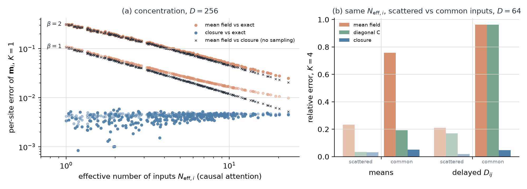
After four updates, shared inputs matter too (see Figure 4(b)). Keeping each coupling row’s weights fixed but moving the large weights onto common columns raises the shared-noise share of $v_i$ (the off-diagonal part of $(JCJ^\top)_{ii}$, averaged over sites) from 1.5% to 37%. Mean field then misses mean overlaps by 76% and delayed correlations by 96%. The diagonal closure reduces the former to 19% but leaves the latter unchanged. The full closure keeps both errors near 5%. The same ordering holds when varying $\beta$ or $u$ separately, with the largest gaps at weak drive.
The stationary state
So far we have only considered one ($K=1$) and four ($K=4$) updates to assess the accuracy of the closure. Let us now look at the long-time relaxation behavior of the dynamics. We use an $N=64$ system with diffuse ($N_{\mathrm{eff}}\approx28$) and sharp ($N_{\mathrm{eff}}\approx4$) couplings. Stationary references use time averages after burn-in from one initialization. For the recursions, we iterate 3000 updates, after which their means change by less than $10^{-16}$ per update.
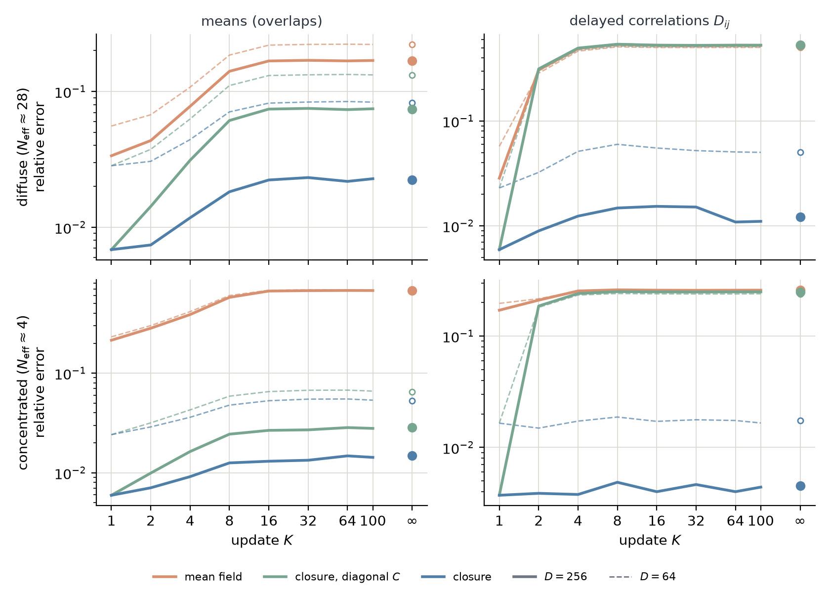
In these runs, the errors grow during the transient but saturate at their stationary values by $K\approx16$, once the dynamics has relaxed, instead of continuing to accumulate. The stationary error decreases with $D$: for diffuse couplings, the closure’s delayed-correlation error falls from 5.1% at $D=64$ to 1.2% at $D=256$. One update is also enough to build the shared covariance that the diagonal closure misses: its delayed-correlation error matches the full closure at $K=1$, but jumps to near mean-field level by $K=2$.
The diffuse system is the previous post’s ensemble. At its operating point $(u,\beta)=(1,1)$, shared covariance resolves the delayed-correlation gap that persisted there. In our tests with nonnegative couplings and nonzero drives, the same holds at lower temperature and weaker drive. The diagonal closure stays at mean-field level throughout, so the gap it leaves grows with $\beta$. At small $D$, the closure can still miss substantially, especially at weak drive. Stationary delayed-correlation errors:
| $(u,\beta)$ | mean field, $D=1024$ | diagonal closure, $D=1024$ | full closure, $D=16$ | $D=64$ | $D=1024$ |
|---|---|---|---|---|---|
| $(1,1)$ | 12% | 12% | 8.8% | 2.2% | 0.13% |
| $(1,2)$ | 54% | 54% | 22% | 5.1% | 0.33% |
| $(1/2,2)$ | 70% | 70% | 42% | 9.1% | 0.42% |
| $(1,4)$ | 91% | 90% | 7.3% | 1.7% | unresolved |
Practical versions
The attentive reader will have noticed the computational cost of the full closure: updating the means costs $O(N^2D)$, like attention, but propagating the dense covariance through $JCJ^\top$ costs $O(N^3)$ per update. There are at least two ways around this:
- For a single update from a product start ($K=1$), the input covariance $C_0$ is diagonal, so the correction has the same asymptotic cost as naive mean field, with one extra $O(N^2)$ pass over the variances.
- For several updates ($K > 1$), we can carry a few random noise channels per site instead of the full matrix, since the means only read the diagonal $v_i=(JCJ^\top)_{ii}$.
A one-step correction (K=1)
From a product start, the spins are independent vMF samples, each in its own initializer field $\mathbf f_j$. In the previous post’s transformer module, for example, these are the values: $\mathbf f_j$ is the $j$-th row of $\mathbf XW_V$. The single-spin response fixes the initial means and variances of the spins:
\begin{equation} \mathbf m_{0,j}=g(\lVert\mathbf f_j\rVert^2)\,\mathbf f_j, \qquad C_{jj}=R^2-\lVert\mathbf m_{0,j}\rVert^2\simeq\frac{2R^2}{1+\gamma(\lVert\mathbf f_j\rVert^2)}. \end{equation}As in Eq. \eqref{eq:first}, only these diagonal variances enter. The update does create off-diagonal covariance, but the first-update means do not need it:
\begin{equation} \bar{\mathbf h}_i=\mathbf x_i+\sum_jJ_{ij}\mathbf m_{0,j}, \qquad v_i=\sum_jJ_{ij}^2C_{jj}, \qquad \mathbf m_i'=g(\lVert\bar{\mathbf h}_i\rVert^2+v_i)\,\bar{\mathbf h}_i. \end{equation}Naive mean field is the same update with $v_i=0$. In code, with drives X of shape (N, D), initializer fields F0 of shape (N, D), couplings J of shape (N, N), inverse temperature beta, and R2 $=R^2$:
import numpy as np

gamma0 = np.sqrt(1 + beta**2 * (F0 * F0).sum(-1) / R2)
M = beta * F0 / (1 + gamma0)[:, None]  # initializer means
var0 = 2 * R2 / (1 + gamma0)  # leading initializer variance, R2 - |M|^2
H = X + J @ M
v = (J * J) @ var0
gamma = np.sqrt(1 + beta**2 * ((H * H).sum(-1) + v) / R2)
M_next = beta * H / (1 + gamma)[:, None]
Zooming out, this resembles a kind of RMSNorm, with the field’s noise variance included in the normalizer (compare the strong-field limit under Norm inflation).
Carrying noise instead of a matrix (K > 1)
Carrying $k$ random noise channels per site reduces the cost of an update from $O(N^2D+N^3)$ to $O(N^2D+kN^2)$. In our experiments, a handful of channels suffices for mean overlaps and aggregate observables, while individual delayed correlations need many more channels or time averaging at stationarity (see Figure 6). We represent the covariance as
\begin{equation} \hat C=\mathrm{diag}(\mathbf b)+\frac1kZZ^\top,\qquad Z\in\mathbb R^{N\times k}, \end{equation}and keep the fresh variance $\mathbf b$ analytic. Set $Y=JZ$ and $v_i=\sum_jJ_{ij}^2b_j+\lVert Y_i\rVert^2/k$, compute the gains as before, and update
\begin{equation} Z'=A\big(Y+J\,\mathrm{diag}(\sqrt{\mathbf b})\,\Xi\big),\qquad b_i'=\frac{2R^2}{1+\gamma_i}, \end{equation}where $\Xi$ has independent standard Gaussian entries. Fresh noise stays diagonal until the couplings mix it across sites. Conditional on the current state, this reproduces the closure’s covariance update in expectation. Later gains depend on sampled noise, so the full trajectory is no longer exactly unbiased (see Appendix D).
Alongside the means and delayed correlations, we also include the aggregate measure $\sigma=\beta\sum_{ij}(J_{ij}-J_{ji})\mathcal D_{ij}$, which, at stationarity, corresponds to the housekeeping entropy production. During relaxation it is only a diagnostic.
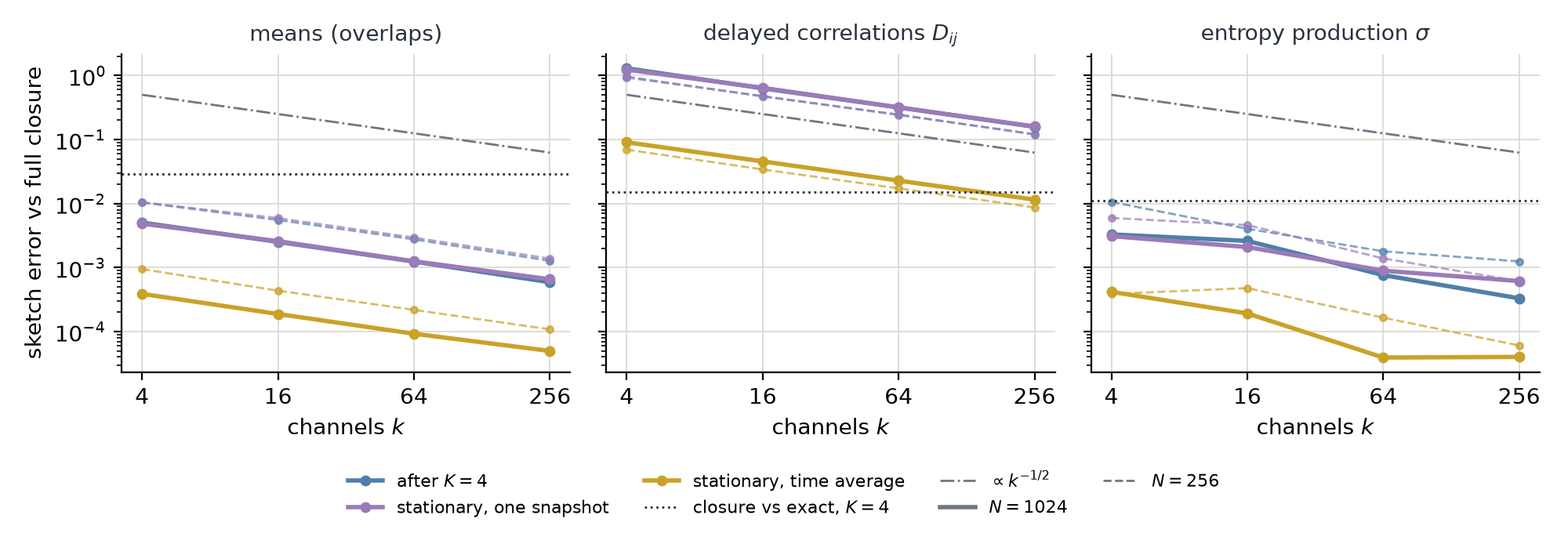
We observe errors falling roughly as $k^{-1/2}$. At $N=1024$, four channels already give mean-overlap errors about six times smaller than the closure’s own error against exact sampling (three to four times at $N=256$), both after four updates and at stationarity. Entropy production, an aggregate over all pairs, also needs only a few channels: at $N=1024$, four already put its error about three times below the closure’s own. Individual delayed correlations are harder: their relative error is about $(2\text{–}2.5)/\sqrt{k}$, requiring $k\sim10^4$ to match the closure here. At stationarity, averaging over 200 updates cuts this error about fourteenfold in these runs, bringing $k\approx64$–$256$ into reach of the closure’s own stationary accuracy.
Relation to other closures
For Ising spins $s_i\in\{-1,1\}$, Mézard and Sakellariou (2011) average the single-spin response over a Gaussian local field:
\begin{equation} \begin{aligned} m_i'&=\mathbb E_z\tanh\!\left[\beta\left(\bar h_i+\sqrt{\Delta_i}\,z\right)\right],\\ \bar h_i&=H_i+\sum_jJ_{ij}m_j, \qquad \Delta_i=\sum_jJ_{ij}^2(1-m_j^2), \end{aligned} \end{equation}where $H_i$ is the external field and $z\sim\mathcal N(0,1)$. Their delayed-covariance relation is
\begin{equation} \mathcal D=\mathrm{diag}(\chi)JC, \qquad \chi_i=\beta\,\mathbb E_z\left\{1-\tanh^2\!\left[\beta\left(\bar h_i+\sqrt{\Delta_i}\,z\right)\right]\right\}. \end{equation}The matrix form matches ours, with a Gaussian-averaged susceptibility $\chi_i$ in place of the gain $a_i$, and $\Delta_i$ matches our diagonal closure’s $v_i=\sum_jJ_{ij}^2C_{jj}$. Huang and Kabashima (2014) keep the correlations between local fields, $\Delta_i=(JCJ^\top)_{ii}$, which matches the full closure and, as in our tests, matters most at low temperature. Their derivations average over Gaussian scalar fields at large $N$ with fully asymmetric couplings. Ours needs no such average, since the gain only sees the field norm, which concentrates at large $D$ for fixed $N$ and $J$. Only the field’s second moments enter.
Aguilera et al. (2021) place Gaussian-field and TAP (Roudi and Hertz, 2011) approximations within a common Plefka framework. Within it, naive mean field and TAP are first- and second-order truncations of an expansion in the coupling strength around independent-spin reference dynamics. Since couplings enter as $\beta J$, these truncations behave like high-temperature expansions, consistent with the growing errors at low temperature in the previous post. Our closure instead uses concentration at large $D$, holding $\beta$ and $J$ fixed, without requiring weak couplings. A direct comparison with second-order Plefka for vector spins remains to be done.
Conclusion and outlook
In this post, we looked at driven vector spins on hyperspheres at fixed couplings as their dimension $D$ grows. Naive mean-field errors level off at a nonzero plateau in this limit: the field’s fluctuations are nearly orthogonal to its mean, so they add a squared length $v_i$ rather than averaging away. We show that the squared field length concentrates at large $D$ around $\lVert\bar{\mathbf h}_i\rVert^2+v_i$, so the gain becomes deterministic. Propagating the covariance that determines $v_i$ then yields a closure for the means and the equal-time and delayed covariance traces.
Numerically, closure errors fall roughly as $1/D$ over the first few updates, and keep improving with $D$ in the stationary states we tested, including at low temperature. Practically, the one-step correction costs one extra pass with squared attention weights, and a few noise channels suffice to accurately capture means over repeated updates. All tests use nonnegative softmax couplings, so signed couplings remain to be checked. At small $D$ or weak drive, the closure errors can still be large.
Now does any of this matter for learning or neural network architecture design? It would be interesting to train a model with corrected one-step modules, or to assess to what extent training simply absorbs the mean-field error. The underlying stochastic system does give us a way to explore modules that sample spins instead of propagating means, and computing couplings from those samples would make the interactions fluctuate too, beyond the fixed-coupling setting here. Passing covariances between layers could preserve information that a mean-only description discards, although the scalar covariance traces tracked here do not capture directional uncertainty.
This concludes our exercise in high-dimensional wobbling.
Acknowledgements
The author (M.B.) would like to thank Á. Poc-López and M. Aguilera for stimulating discussions.
AI tool use. This project was a personal experiment in agentic research with human steering. Claude Opus 5.5 and GPT-6 Astra participated in brainstorming, experimental design, coding, writing assistance, figure generation, and multiple rounds of adversarial reviewing using their respective native coding harnesses. Tactical decisions were impressive, but strategic manoeuvres and taking leaps proved harder than expected, requiring significant steering. Multiple rounds of manual revision and editing were required. Any remaining slop is entirely the responsibility of the author (M.B.).
References
If you happen to find this work useful, please consider citing it as:
@article{bal2026largedclosure,
  title   = {A Large-D Closure for Asymmetric Kinetic Vector-Spin Systems},
  author  = {Bal, Matthias},
  year    = {2026},
  month   = {October},
  url     = {https://mcbal.github.io/post/a-large-d-closure-for-asymmetric-kinetic-vector-spin-systems/}
}
- M. Bal, Spin-Model Transformers and Nonequilibrium Dynamics in Spin-Model Transformers, with mcbal/neqnn.
- M. Aguilera, S. A. Moosavi, H. Shimazaki, A unifying framework for mean-field theories of asymmetric kinetic Ising systems, Nat. Commun. 12, 1197 (2021); arXiv:2002.04309.
- M. Mézard, J. Sakellariou, Exact mean-field inference in asymmetric kinetic Ising systems, J. Stat. Mech. L07001 (2011).
- Y. Roudi, J. Hertz, Dynamical TAP equations for non-equilibrium Ising spin glasses, J. Stat. Mech. P03031 (2011).
- H. Huang, Y. Kabashima, Dynamics of asymmetric kinetic Ising systems revisited, J. Stat. Mech. P05020 (2014).
- H. E. Stanley, Spherical model as the limit of infinite spin dimensionality, Phys. Rev. 176, 718 (1968).
- A. T. A. Wood, Simulation of the von Mises–Fisher distribution, Commun. Stat. Simul. Comput. 23, 157–164 (1994).
Appendices
Appendix A: The geometry of a high-dimensional vMF
Write a unit sample as $\mathbf u=t\hat{\mathbf h}+\sqrt{1-t^2}\,\boldsymbol\xi$, where $\boldsymbol\xi$ is uniform on the transverse unit sphere and independent of $t$. The alignment density is
\begin{equation} p(t)\propto\underbrace{e^{\kappa t}}_{\text{alignment}}\;\underbrace{(1-t^2)^{(D-3)/2}}_{\text{room to fluctuate}},\qquad -1\lt t\lt1. \end{equation}At fixed $\kappa/D$, maximizing the leading log density gives the typical latitude; its curvature gives the width:
\begin{equation} t_\star=\frac{\kappa}{D/2+\sqrt{D^2/4+\kappa^2}}, \qquad \operatorname{std}(t)\simeq\frac{1-t_\star^2}{\sqrt{D(1+t_\star^2)}}. \end{equation}The exact mean alignment is $A_D(\kappa)=t_\star+O(1/D)$. With $\kappa=\beta R\lVert\mathbf h\rVert$ and $R^2=D/2-1$, this recovers $t_\star\simeq\lVert g(\lVert\mathbf h\rVert^2)\,\mathbf h\rVert/R$, the leading-order response of Eq. \eqref{eq:response}. The most likely latitude stays away from the pole, even though the pole maximizes the density per unit area.
The transverse length remains finite, but its projection onto any fixed unit vector has standard deviation at most $1/\sqrt{D-1}$. For $n$ independent samples from the same vMF,
\begin{equation} \mathbb E\lVert\bar{\mathbf u}\rVert^2=A_D(\kappa)^2+\frac{1-A_D(\kappa)^2}{n}. \end{equation}Averaging divides the noise’s expected squared length by $n$; as $D$ grows at fixed $n$ and $\kappa/D$, that expected squared length approaches a nonzero limit.
Appendix B: Covariance of a vMF spin
For $\kappa=\beta R\lVert\mathbf h\rVert$, the exact mean is $\boldsymbol\mu_D=R A_D(\kappa)\hat{\mathbf h}$. The covariance separates into transverse and longitudinal parts:
\begin{equation} \Sigma(\mathbf h)=\tau(I-\hat{\mathbf h}\hat{\mathbf h}^\top)+\rho\hat{\mathbf h}\hat{\mathbf h}^\top, \end{equation}\begin{equation} \tau=\frac{R^2A_D(\kappa)}{\kappa}, \qquad \rho=R^2\left(1-\frac{(D-1)A_D(\kappa)}{\kappa}-A_D(\kappa)^2\right). \end{equation}At zero field, $\boldsymbol\mu_D=0$ and $\Sigma=(R^2/D)I$. Two useful exact identities are $\boldsymbol\mu_D=\beta\tau\mathbf h$ and $\partial\boldsymbol\mu_D/\partial\mathbf h=\beta\Sigma$: fluctuations determine the response to a small change in field.
At fixed $\beta\lVert\mathbf h\rVert/R$,
\begin{equation} \tau=\frac{1}{1+\gamma}+O(1/D), \qquad \rho=\frac{1}{\gamma(1+\gamma)}+O(1/D), \qquad \gamma=\sqrt{1+\beta^2\lVert\mathbf h\rVert^2/R^2}. \end{equation}Every directional variance stays $O(1)$. The longitudinal variance is smaller by a factor $\gamma$ to leading order, but occupies only one direction. Summing all $D$ directions gives the fresh variance used in the closure:
\begin{equation} \operatorname{tr}\Sigma=R^2\bigl[1-A_D(\kappa)^2\bigr]\simeq\frac{2R^2}{1+\gamma}. \end{equation}Appendix C: Why the field norm concentrates
Fix $N$, $J$, $\beta$ and the number of updates, take drives of length $O(R)$, and start from independent vMF spins. Every squared field length is determined by the overlaps
\begin{equation} Q_{ij}=\frac{\mathbf s_i\cdot\mathbf s_j}{R^2}, \qquad U_{ij}=\frac{\mathbf x_i\cdot\mathbf s_j}{R^2}, \end{equation}namely
\begin{equation} \frac{\lVert\mathbf h_i\rVert^2}{R^2} =\frac{\lVert\mathbf x_i\rVert^2}{R^2} +2\sum_jJ_{ij}U_{ij} +\sum_{jl}J_{ij}J_{il}Q_{jl}. \end{equation}It is enough to show that every overlap has variance $O(1/D)$, so that its fluctuations are $O(D^{-1/2})$. Since $Q_{ii}=1$ exactly, only overlaps between distinct sites, and with drives, need checking. We proceed one update at a time.
Independent spins. Write $\mathbf s_i=\mathbf m_i+\delta\mathbf s_i$ with independent fluctuations of covariance $\Sigma_i$. A vMF spin has $O(1)$ variance along any direction, while its total variance is at most $R^2$. For distinct sites, the fluctuating parts of $R^2Q_{ij}$ are $\mathbf m_i\cdot\delta\mathbf s_j$, $\delta\mathbf s_i\cdot\mathbf m_j$ and $\delta\mathbf s_i\cdot\delta\mathbf s_j$, with variances
\begin{equation} \mathbf m_i^\top\Sigma_j\mathbf m_i=O(D), \qquad \mathbf m_j^\top\Sigma_i\mathbf m_j=O(D), \qquad \operatorname{tr}(\Sigma_i\Sigma_j)=O(D). \end{equation}Dividing by $R^4$ gives variance $O(1/D)$. The drive overlaps $U_{ij}$ only involve the first kind of term.
One update. Given the current spins, the next spins are $\mathbf s_i'=\boldsymbol\mu_D(\mathbf h_i)+\boldsymbol\epsilon_i$, where the fresh noise is independent across sites, has zero mean, and again has $O(1)$ variance along any direction. The next overlap between distinct sites splits into a conditional mean and noise:
\begin{equation} Q_{ij}'=\frac{\boldsymbol\mu_D(\mathbf h_i)\cdot\boldsymbol\mu_D(\mathbf h_j)}{R^2} +\frac{\boldsymbol\mu_D(\mathbf h_i)\cdot\boldsymbol\epsilon_j+\boldsymbol\epsilon_i\cdot\boldsymbol\mu_D(\mathbf h_j)+\boldsymbol\epsilon_i\cdot\boldsymbol\epsilon_j}{R^2}. \end{equation}The noise term has conditional variance $O(1/D)$, by the same calculation as for independent spins, with the conditional means in place of $\mathbf m_i$. To control the conditional mean, write the leading gain in terms of the normalized squared field length:
\begin{equation} G(q)=\frac{\beta}{1+\sqrt{1+\beta^2q}}, \qquad q_i=\frac{\lVert\mathbf h_i\rVert^2}{R^2}. \end{equation}Up to a uniform $O(1/D)$ correction on the bounded field range, the conditional mean of $Q_{ij}'$ is $G(q_i)G(q_j)\,\mathbf h_i\cdot\mathbf h_j/R^2$. Both $G$ and its derivative are bounded for $q\geq0$. The quantities $q_i$ and $\mathbf h_i\cdot\mathbf h_j/R^2$ are linear combinations of the current overlaps and fixed drive overlaps. Since these overlaps are bounded, the leading conditional mean has bounded derivatives with respect to them, uniformly in $D$. A function with bounded derivatives of a fixed number of variables with variance $O(1/D)$ also has variance $O(1/D)$; the uniform response correction does not change this order. By the law of total variance,
\begin{equation} \operatorname{Var}Q_{ij}' =\mathbb E\operatorname{Var}(Q_{ij}'\mid\mathbf S) +\operatorname{Var}\mathbb E(Q_{ij}'\mid\mathbf S) =O(1/D). \end{equation}The same argument applies to $U_{ij}'$, which completes the step. Spins correlated by shared inputs are no obstacle: only the fresh noise needs to be independent, and it is, given the current spins.
This establishes concentration at any fixed number of updates. The constants can compound from step to step and grow with $N$ and the couplings, so stationary accuracy needs a separate check.
Size of the residual
Eq. \eqref{eq:linear} becomes exact once we add the residual $\mathbf e_i=\boldsymbol\mu_D(\mathbf h_i)-a_i\mathbf h_i$. It has two parts:
- The finite-$D$ response, $\boldsymbol\mu_D(\mathbf h_i)-g(\lVert\mathbf h_i\rVert^2)\,\mathbf h_i$: a relative $O(1/D)$ correction to a vector of length $O(\sqrt D)$, so its length is $O(D^{-1/2})$.
- The fluctuating gain, $\bigl[g(\lVert\mathbf h_i\rVert^2)-g(r_i^2)\bigr]\mathbf h_i\approx g'(r_i^2)\,\Delta_i\mathbf h_i$ with $\Delta_i=\lVert\mathbf h_i\rVert^2-r_i^2$. Since $g'=O(1/D)$, $\Delta_i$ has root-mean-square size $O(\sqrt D)$ by the concentration shown above, and $\lVert\mathbf h_i\rVert=O(\sqrt D)$, this contribution has root-mean-square length $O(1)$.
The residual shifts the mean by at most $O(1)$ and adds a fluctuation of root-mean-square length $O(1)$, against a spin length $R=O(\sqrt D)$. At a fixed number of updates, this bounds the absolute errors in $\mathbf m_i/R$, $C_{ij}/R^2$ and $\mathcal D_{ij}/R^2$ by $O(D^{-1/2})$. The $1/D$ decay we observe numerically is faster than this bound.
Appendix D: The sampled closure
Split $C=\mathrm{diag}(\mathbf b)+S$ into the last update’s fresh variance and older noise. Fresh variance is diagonal; older noise has passed through $J$ and is correlated across sites. Represent it by $S\approx ZZ^\top/k$, with $k$ channels per site. For a product start, initialize $Z_0=0$ and $b_{0,i}=R^2-\lVert\mathbf m_{0,i}\rVert^2$.
Why a few channels suffice. Fresh variance needs only one number per site. Once the couplings spread it across sites, random channels carry the resulting correlations through the same matrix multiplication as the means.
At each update, draw a new $\Xi\in\mathbb R^{N\times k}$ with independent standard Gaussian entries, independently of the current state and all previous draws, and set
\begin{equation} Z'=AJ\big(Z+\mathrm{diag}(\sqrt{\mathbf b})\,\Xi\big), \qquad b_i'=\frac{2R^2}{1+\gamma_i}. \end{equation}Since $\mathbb E\Xi=0$ and $\mathbb E\Xi\Xi^\top=kI$,
\begin{equation} \mathbb E\!\left[\tfrac1kZ'Z'^\top\,\middle|\,\mathbf m,Z,\mathbf b\right] =AJ\Big(\tfrac1kZZ^\top+\mathrm{diag}(\mathbf b)\Big)J^\top A =AJ\hat CJ^\top A. \end{equation}Adding $\mathrm{diag}(\mathbf b')$ reproduces the closure’s update applied to the current $\hat C$. From a product start, $Z=0$, so the first gains, means and delayed correlations match the full closure. The new off-diagonal covariance is already sampled.
With $Y=JZ$, the required quantities are
\begin{equation} v_i=\sum_jJ_{ij}^2b_j+\frac{\lVert Y_i\rVert^2}{k}, \qquad \hat{\mathcal D}=A\left(J\,\mathrm{diag}(\mathbf b)+\frac{YZ^\top}{k}\right). \end{equation}Evolution costs $O(N^2D+kN^2)$ and adds $O(Nk)$ covariance storage. Dense $C$ or $\mathcal D_{ij}$ readouts can be formed when needed; the stationary entropy-production estimate $\hat\sigma^\star=\beta\sum_{ij}(J-J^\top)_{ij}\hat{\mathcal D}_{ij}^\star$ can be computed directly from the factors. In attention terms, $Z$ adds $k$ value channels under the same weights.
Channel fluctuations scale roughly as $k^{-1/2}$. Gains and aggregate observables can average over many sites as well; an individual delayed correlation remains one sampled inner product. This explains their different accuracies in Figure 6.
Later gains depend on sampled $v_i$, so the full trajectory is not exactly unbiased. An $O(1/k)$ bias is plausible from a second-order expansion, but has not been established. The sphere identity holds conditionally in expectation at each update. In Figure 6, the per-site variance misses $R^2-\lVert\mathbf m_i\rVert^2$ by $3$–$5\%$ of $R^2$ at $k=4$ and under $1\%$ at $k=256$, without renormalization.
At stationarity, fresh channel draws can make time averaging useful, but successive states still share propagated noise. The benefit of time averaging depends on temporal autocorrelation. Averaging 200 updates reduced delayed-correlation error about fourteenfold in these runs, mean-overlap error by 11–14 times, and entropy-production error by 7–23 times. These are empirical reductions, not a general effective-sample-size rule.
Footnotes
Scaling $R^2\propto D$ follows the large-component convention for vector spins (Stanley 1968). The choice $R^2=D/2-1$ also matches the Bessel order appearing in vMF means and simplifies their leading-order formulas. In units of $R$, the leading response depends only on $\beta\lVert\mathbf h\rVert/R$. ↩︎
Appendix C makes this precise at any fixed number of updates. ↩︎
Up to a residual whose size is bounded in Appendix C. ↩︎
Reference moments use exact vMF sampling (Wood, 1994) over independent replicates. Squared errors are formed from products across distinct replicates, which cancels Monte Carlo variance in expectation. Intervals show two jackknife standard errors, leaving out one replicate at a time. ↩︎
